O Level Business: Costs, scale of production and break-even analysis (Cambridge 7115)

This guide is aligned to the Cambridge O Level Business Studies 7115 syllabus for examination in 2026. It covers section 4.2, Costs, scale of production and break-even analysis, which sits inside Operations management. Costs and break-even work can appear on Paper 1 (short answer and data response) and on Paper 2 (case study), so you need both the calculations and the written reasoning.

For fast recall use the revision notes. To test yourself use the practice questions. The rest of the topic (production methods, location) is in the operations management practice set. Course pages: Cambridge O Level Business hub and the printable checklist. Unsure where you stand? Try the free 10-minute diagnostics.

What the syllabus asks for

Section	What you must be able to do
4.2.1	Identify and classify costs (fixed, variable, average, total) and use cost data to make simple cost-based decisions, such as stopping production or continuing
4.2.2	Explain economies of scale (purchasing, marketing, financial, managerial, technical) and diseconomies of scale (poor communication, lack of commitment from employees, weak coordination)
4.2.3	Explain break-even; construct, complete or amend a simple chart; interpret a chart; calculate break-even output; define, calculate and interpret margin of safety; use break-even for simple decisions such as a higher price; understand its limitations

All money in this guide is in dollars. Every business is invented.

4.2.1 Identify and classify costs

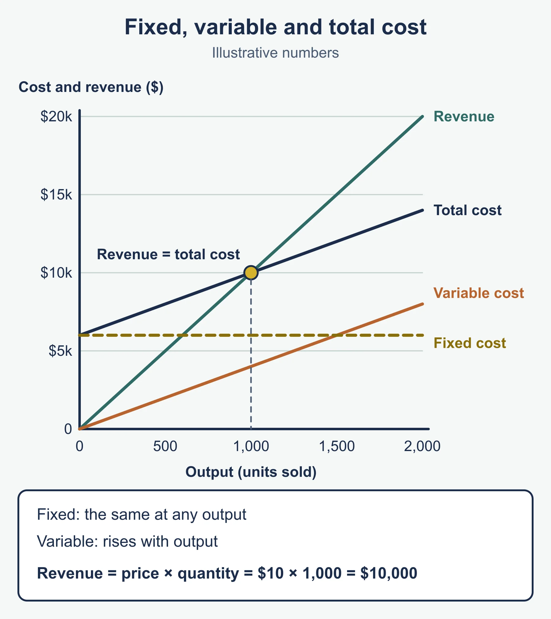
Fixed costs do not change when output changes, within the range the business normally works in. Rent, insurance and managers’ salaries are typical. Variable costs change directly with output: raw materials, packaging and the wages of workers paid per item. Total cost is fixed costs plus variable costs. Average cost (also called cost per unit) is total cost divided by the number of units produced. The syllabus gives these four as examples, so learn a definition and a formula for each.

Cost	How to find it
Total variable cost	variable cost per unit x output
Total cost	fixed costs + total variable cost
Average cost	total cost / output

Worked example: classifying and calculating

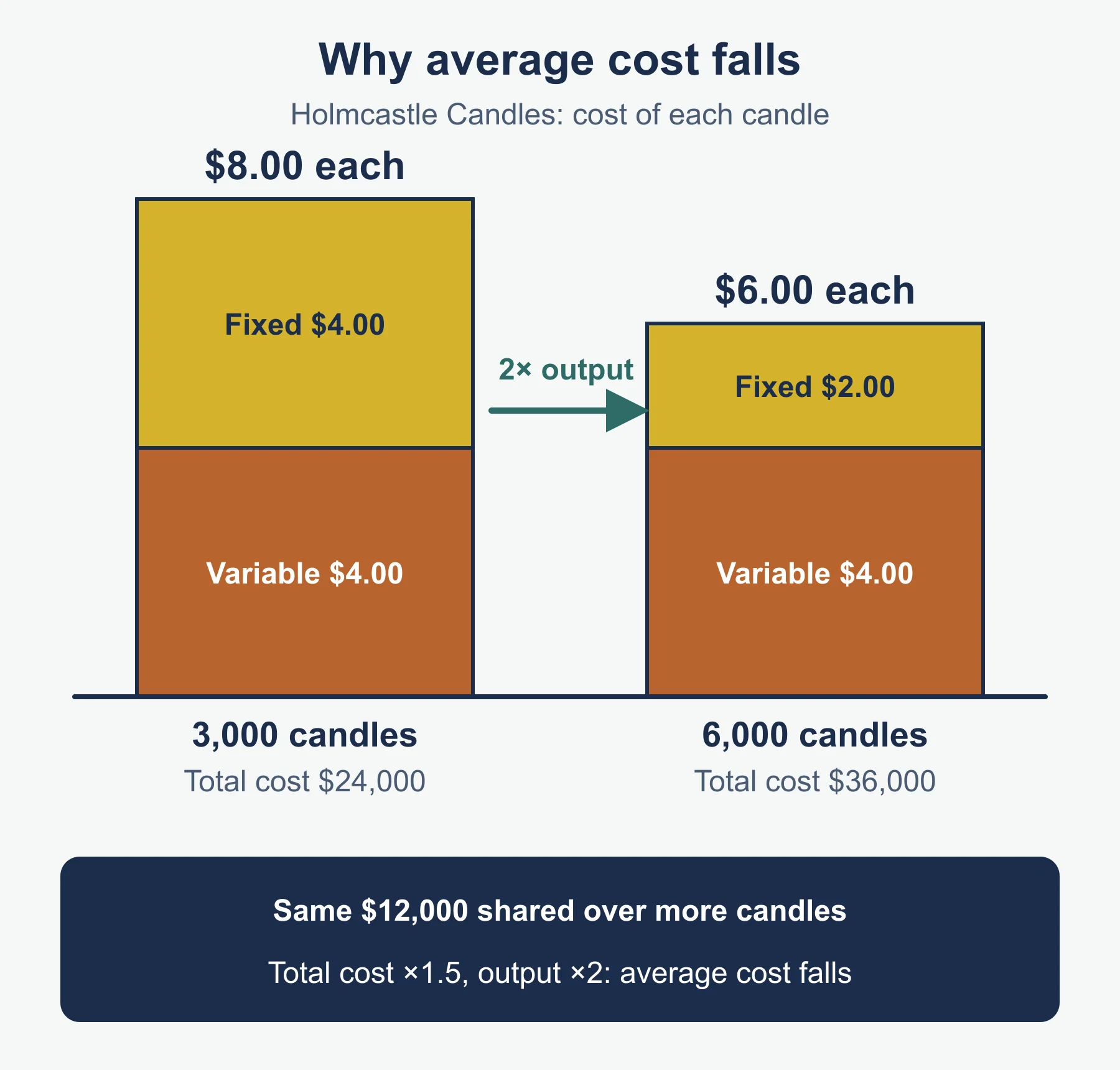
Holmcastle Candles pays rent of 6 000, insurance of 1 000 and salaries of 5 000 each month. These are fixed, so fixed costs are 12 000. Each candle needs wax (1.50), a jar (0.90) and labour (1.60). Variable cost per candle is 1.50 + 0.90 + 1.60 = 4.00.

Output	Total variable cost	Total cost	Average cost
3 000	12 000	24 000	8.00
6 000	24 000	36 000	6.00

Total cost rose by half, but output doubled. Average cost fell because the same 12 000 of fixed costs is shared over more candles (4.00 per candle at 3 000 units, 2.00 at 6 000). This is why higher output often lowers average cost.

Cost-based decisions: stop or continue?

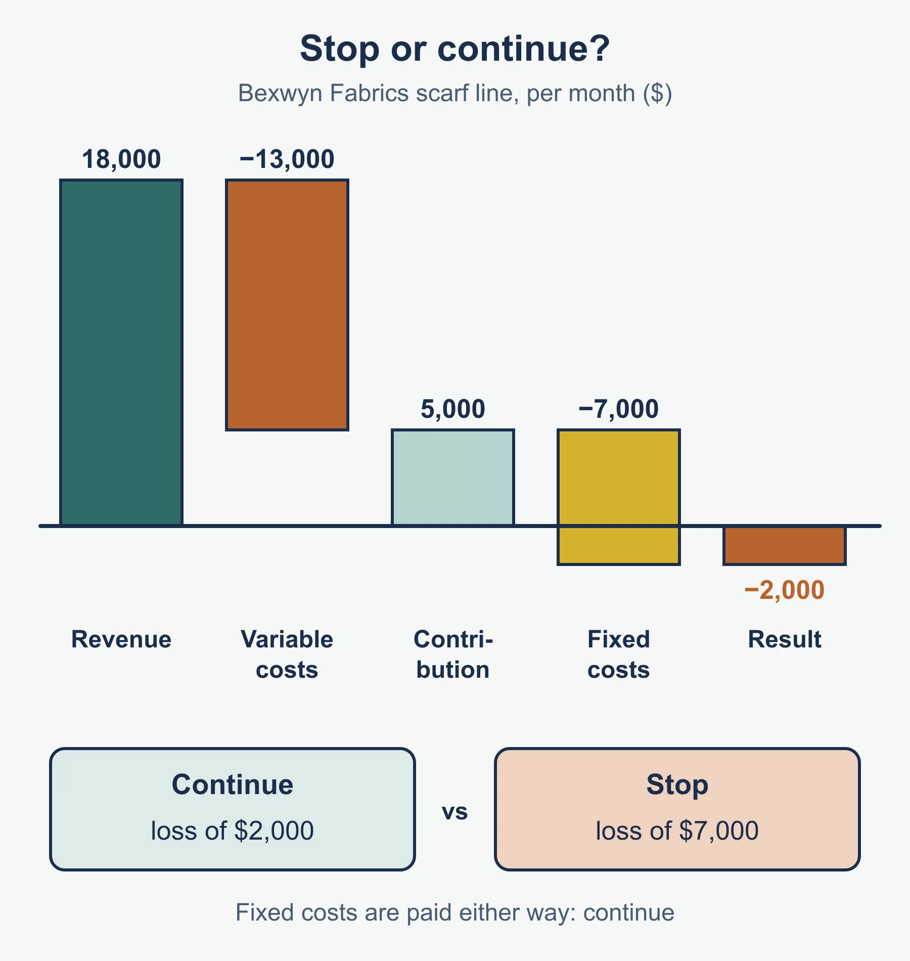
A business may ask whether a product that shows a loss should be dropped. The key question is which costs go away if production stops. Variable costs stop. Fixed costs often do not, at least in the short run. So compare the revenue from the product with its variable costs. If revenue is higher, the product makes a contribution (revenue minus variable costs) towards fixed costs, and stopping makes the business worse off. This is the standard way to approach the decision; the syllabus only asks for simple cost-based decisions.

Worked example: the scarf line

Bexwyn Fabrics sells 2 000 scarves a month at 9 each. Variable cost is 6.50 per scarf. Fixed costs of 7 000 a month are charged to the scarf line, and the firm pays them whether or not scarves are made.

• Revenue = 2 000 x 9 = 18 000
• Variable costs = 2 000 x 6.50 = 13 000
• Contribution = 18 000 - 13 000 = 5 000
• Loss if it continues = 5 000 - 7 000 = a loss of 2 000
• Loss if it stops = 0 - 7 000 = a loss of 7 000

Continuing loses 2 000; stopping loses 7 000. The scarf line should continue for now. A good answer adds that this changes if the fixed costs could be avoided, if the money could earn more elsewhere, or if the contribution will turn negative.

4.2.2 Economies and diseconomies of scale

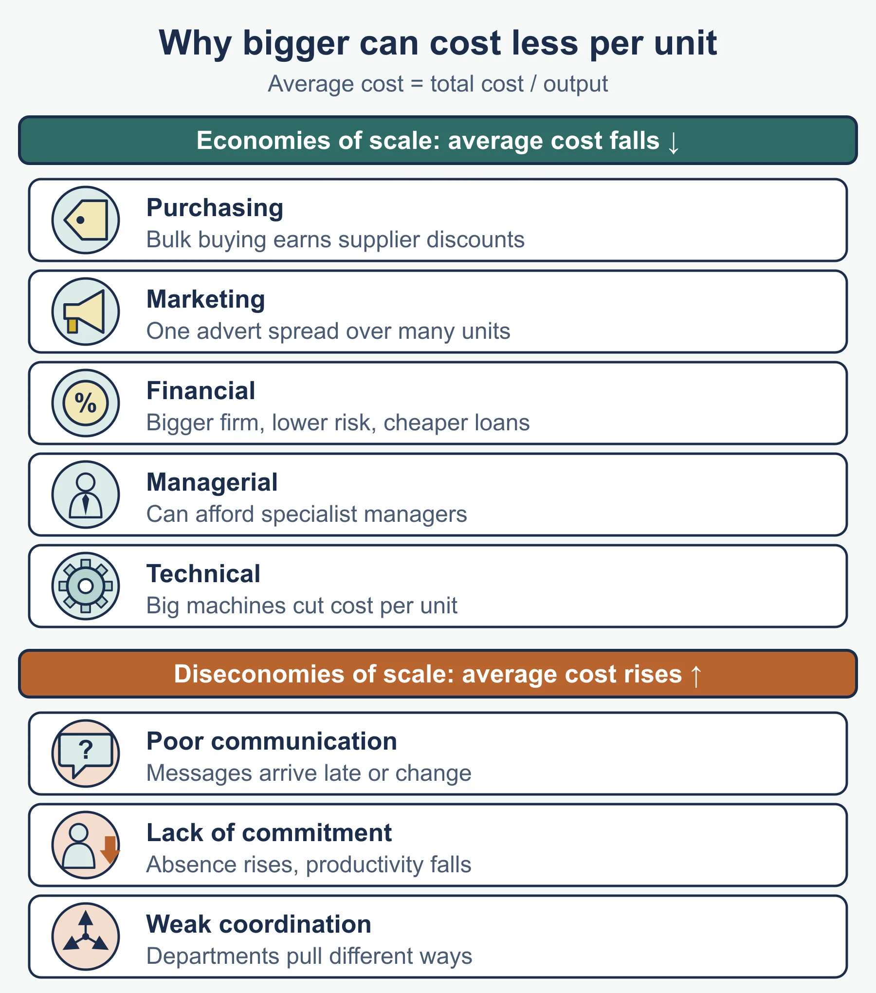
Economies of scale are the cost advantages that let average cost fall as a business increases its scale of production. They are not simply “lower costs”: the saving is in cost per unit.

Type	How average cost falls	Example
Purchasing	Bulk buying earns discounts from suppliers	A juice maker buys fruit by the lorry load at a lower price per kilo
Marketing	The cost of advertising is spread over more units	One TV advert supports a very large sales volume
Financial	Larger firms are seen as lower risk, so banks may charge lower interest	A bigger firm borrows at a cheaper rate
Managerial	Large firms can afford specialist managers who work more efficiently	A full-time finance director replaces the owner doing the accounts
Technical	Large machines, or a production line, lower cost per unit but only pay off at high output	A high-speed bottling line

Diseconomies of scale are the rise in average cost that can happen when a business becomes too large.

• Poor communication. Messages pass through many layers, arrive late or change on the way, so mistakes and delays cost money.
• Lack of commitment from employees. Workers in a very large firm may feel unimportant, so absence and labour turnover rise and productivity falls.
• Weak coordination. Many departments or sites pull in different directions, which causes duplication and delays.

Worked example: a cost curve

Pellbright Juice records these results (all amounts in dollars).

Output (litres)	Total cost	Average cost
10 000	12 000	1.20
20 000	19 000	0.95
40 000	32 000	0.80
80 000	68 000	0.85
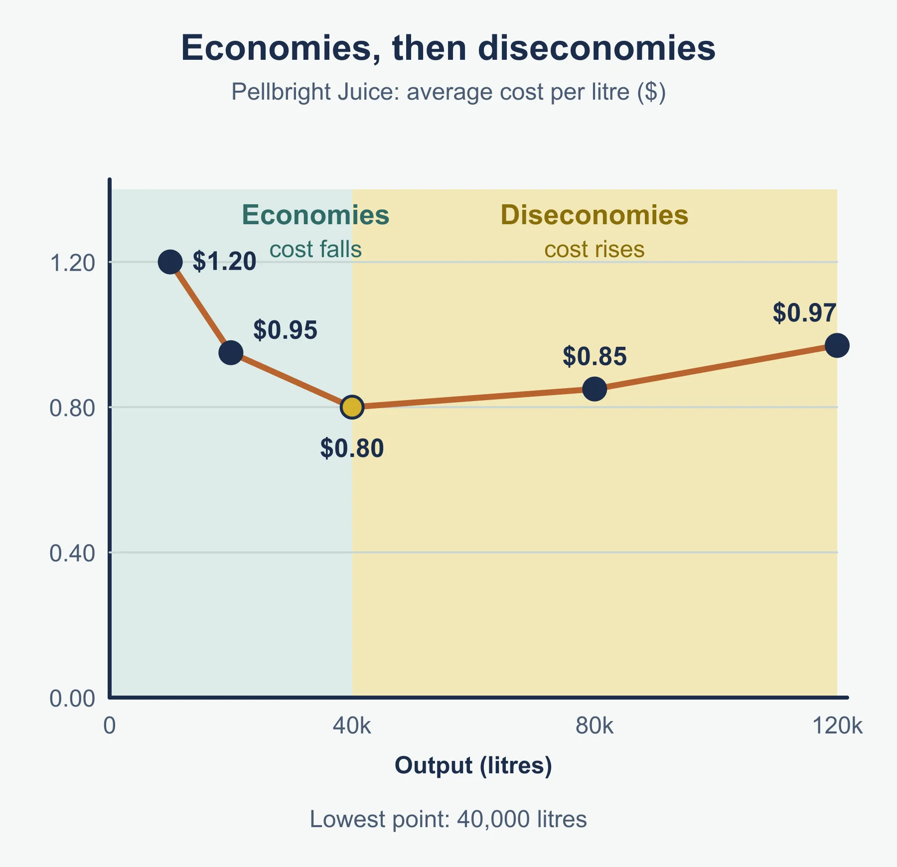
120 000	116 400	0.97

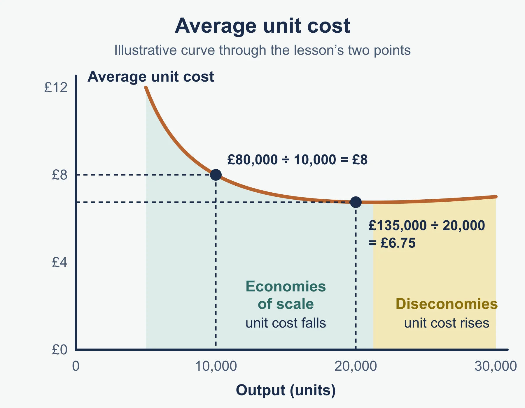
Average cost falls from 1.20 to 0.80 as output rises to 40 000 litres: economies of scale, such as bulk fruit discounts and a faster filling machine. After 40 000 it rises, to 0.97 at 120 000 litres. This points to diseconomies, perhaps because supervisors cannot coordinate three shifts. Draw average cost against output and you get a U shape: it falls, bottoms out, then rises.

4.2.3 Break-even analysis

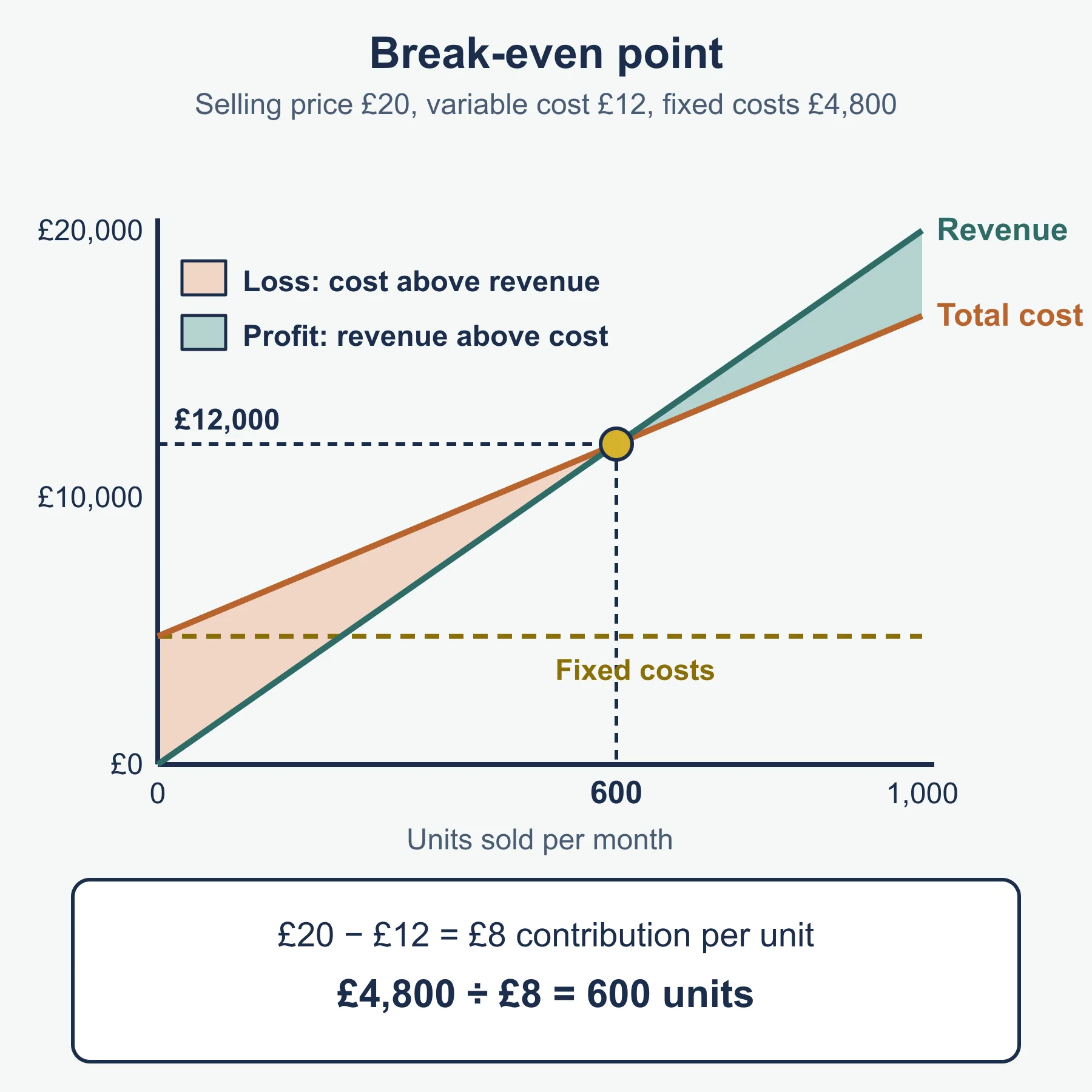
Break-even is the point where a business sells enough for total revenue to equal total cost, so it makes neither profit nor loss. Below it there is a loss; above it there is a profit.

Two standard forms are used. The syllabus does not print formulas for them, so these are the standard forms:

• Contribution per unit = selling price per unit - variable cost per unit
• Break-even output = fixed costs / contribution per unit

Worked example: break-even output

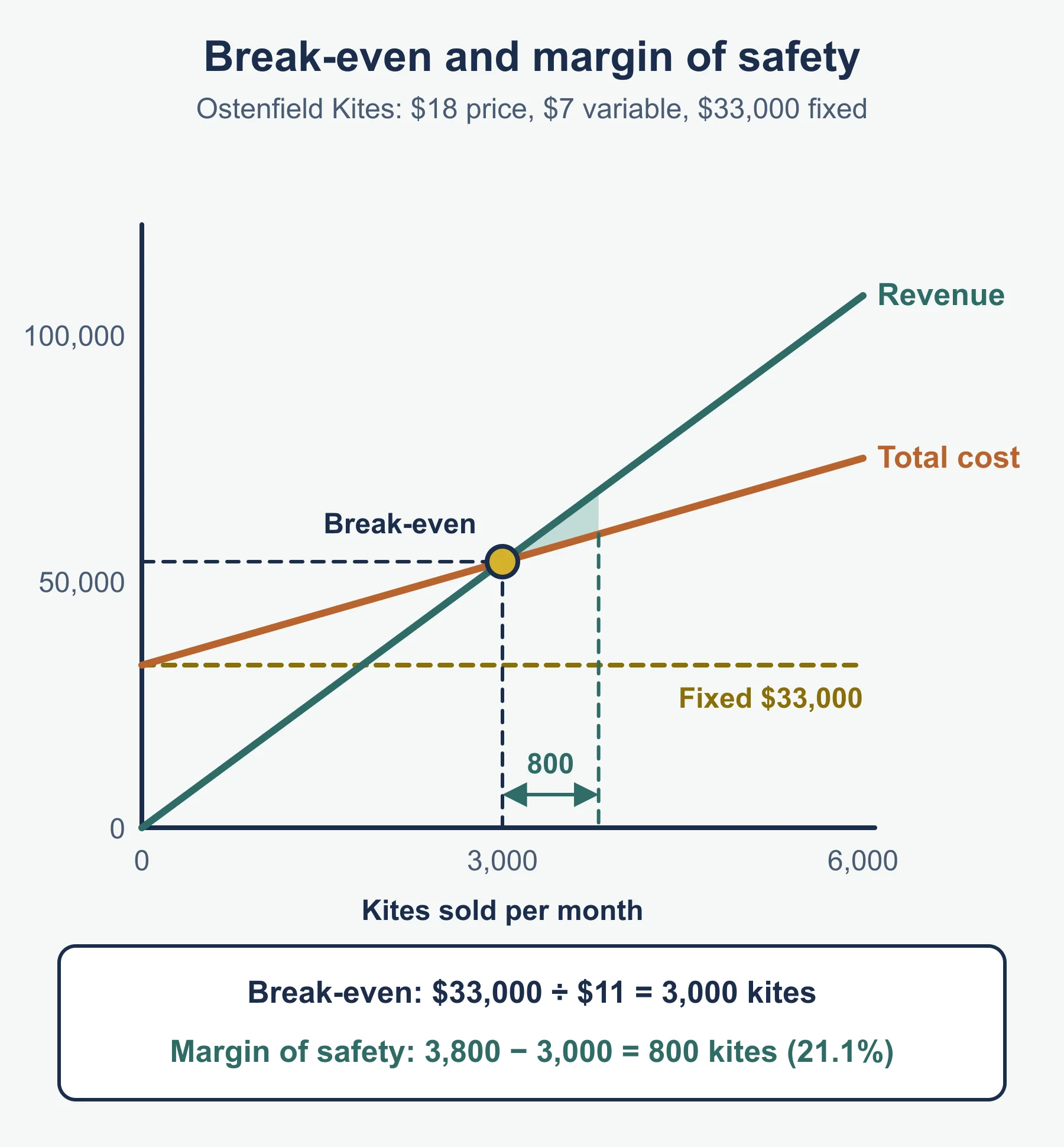
Ostenfield Kites sells kites at 18 each. Variable cost is 7 per kite and fixed costs are 33 000 a month.

• Contribution per unit = 18 - 7 = 11
• Break-even output = 33 000 / 11 = 3 000 kites

Check: revenue 3 000 x 18 = 54 000; total cost 33 000 + 3 000 x 7 = 54 000. They match.

Constructing, completing or amending a chart

A simple break-even chart puts output along the horizontal axis and money (for both costs and revenue) up the vertical axis. Three lines are drawn.

1. Fixed costs: a horizontal line at 33 000.
2. Total costs: starts at 33 000 on the vertical axis (zero output) and rises. Plot a second point, for example at 6 000 kites: 33 000 + 6 000 x 7 = 75 000.
3. Total revenue: starts at the origin and rises more steeply. At 6 000 kites it is 6 000 x 18 = 108 000.

Where total revenue crosses total costs is break-even, at 3 000 kites. Two points per line are enough, and a ruler makes the lines straight.

Money
  ^                       / Revenue
  |                     /   . Total costs
  |                   /  .
  |                 X
  |             . /    <- X = break-even
  |  FC ----.------------------- fixed costs
  |    .  /
  +---------------------------> Output

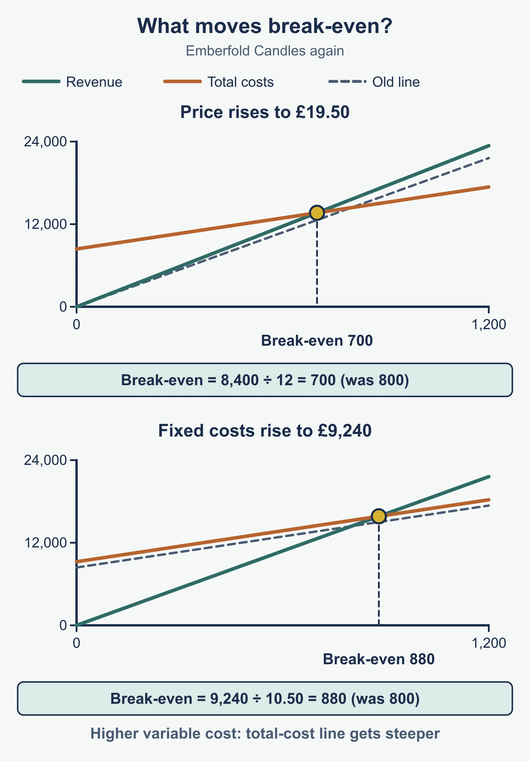
To amend a chart when something changes, move the right line. Higher rent lifts the fixed cost line and the total cost line by the same amount, so break-even moves right. A higher price makes the revenue line steeper, so break-even moves left. Lower variable cost per unit makes the total cost line less steep, so break-even also moves left.

Margin of safety

The margin of safety is how far sales (or output) are above the break-even level. It shows how far sales can fall before the business makes a loss.

• Margin of safety (units) = actual or expected output - break-even output
• As a percentage = margin of safety / actual or expected output x 100 (standard form)

If Ostenfield expects to sell 3 800 kites: 3 800 - 3 000 = 800 kites, or 800 / 3 800 x 100 = 21.1% of expected sales. On the chart it is the gap between break-even and the actual output, measured along the output axis. A large margin means the business has more protection if demand falls.

Using break-even to help decisions

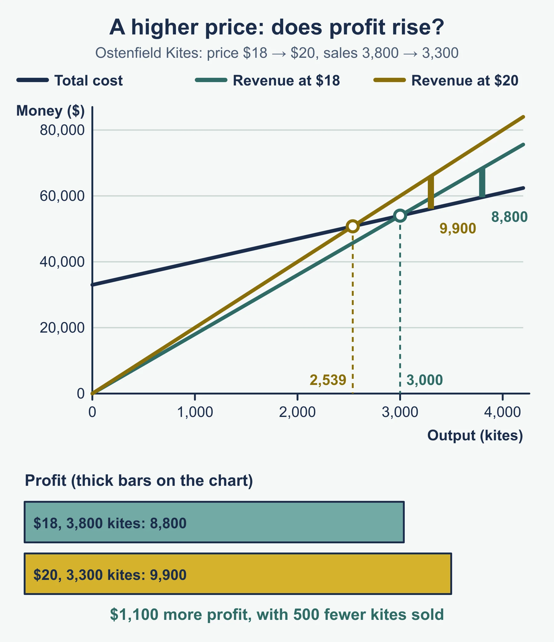
Suppose Ostenfield raises the price to 20, but expects sales to fall to 3 300 kites.

• New contribution = 20 - 7 = 13
• New break-even = 33 000 / 13 = 2 538.46, so about 2 539 kites
• Profit at 3 300 kites = 13 x 3 300 - 33 000 = 9 900
• Profit at the old price and 3 800 kites = 11 x 3 800 - 33 000 = 8 800

The higher price lowers break-even and raises profit, even with fewer sales. A justified answer also notes that the result depends on the forecast fall in demand. If sales dropped much further, the decision would look different.

Limitations of break-even analysis

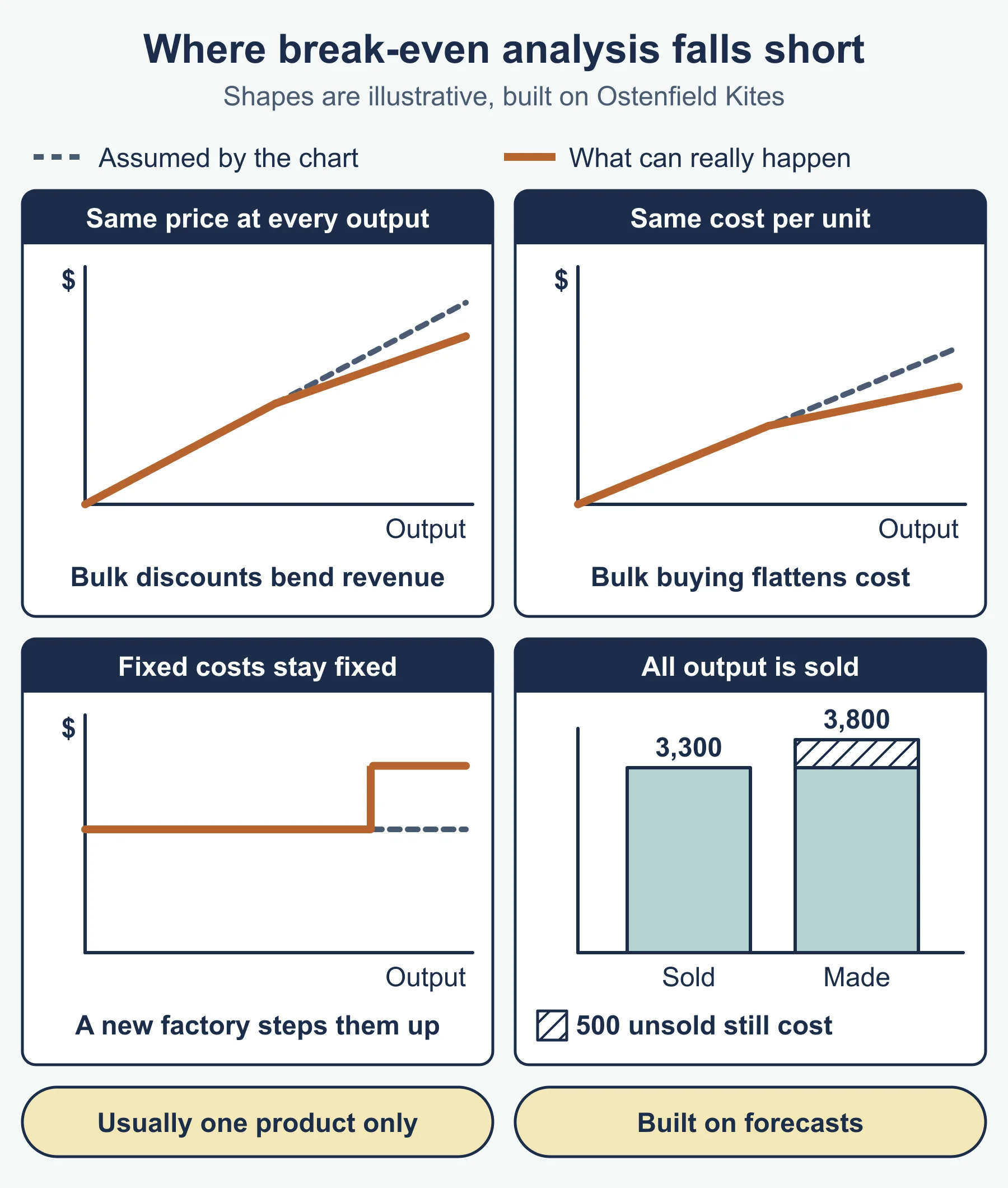
• It assumes all output is sold. Unsold stock still costs money.
• It assumes the selling price stays the same at every output, so discounts for bulk orders are ignored.
• It assumes variable cost per unit is constant. Bulk buying (a purchasing economy) would change it.
• Fixed costs are treated as fixed, but at high output a business may need a new factory.
• It is usually drawn for one product, but many firms sell several.
• It depends on forecasts, which can be wrong, and it is a snapshot that ignores competitors’ reactions.

Common errors

• Dividing fixed costs by the selling price instead of contribution per unit.
• Writing “costs fall” instead of “average cost falls” for economies of scale.
• Putting the fixed cost line through the origin on a chart. It starts above zero on the vertical axis.
• Calling a benefit a type of economy without linking it to cost per unit.
• Stopping a product because it shows a loss without checking the contribution.
• Giving margin of safety in money when the question gave units, or leaving out units.

Frequently asked questions

What is the difference between fixed and variable costs? Fixed costs, such as rent, insurance and managers’ salaries, do not change when output changes within the normal range. Variable costs, such as raw materials and packaging, change directly with output.

Should a business stop making a product that shows a loss? Not necessarily. If fixed costs would still be paid after stopping, the product may lose less by continuing as long as it makes a positive contribution, so check which costs would actually go away.

What are the main diseconomies of scale? Poor communication through many layers, lack of commitment from employees in a very large firm, and weak coordination between departments or sites. Each can raise average cost as a business grows too large.

Why does average cost fall as output rises? Fixed costs are shared over more units, so the fixed cost per unit falls. Economies of scale, such as bulk-buying discounts and faster machines, can lower average cost further.

Official syllabus

Source: Cambridge O Level Business Studies 7115 syllabus for examination in 2026, published by Cambridge International, section 4.2.