Time Series and Moving Averages: O Level Statistics 4040 and IGCSE 0479 Revision Notes

These revision notes cover time series for Cambridge O Level Statistics 4040, syllabus sections 10.1 (understanding of trend) and 10.2 (understanding of seasonal variation), from the syllabus for examination in 2025, 2026 and 2027. The same content is tagged to the time series topic of Cambridge IGCSE Statistics 0479. For full explanations start with the time series study guide, then test yourself with the practice questions.

Useful links: Cambridge O Level Statistics hub, printable checklist and the free 10-minute diagnostics. Related topic: index numbers.

What the syllabus lists

Section	Official wording	What it means for you
10.1	Understanding of trend, including determination by calculation of moving averages, with centring, where appropriate	Say what a trend is, calculate moving averages, centre them when the number of points is even, and draw the trend
10.2	Understanding of seasonal variation, including calculation of mean seasonal variation	Find how far each season sits above or below the trend, on average
10.2	Use of a trend line and seasonal component in prediction	Combine a trend value with a seasonal component to predict a future value
0479 topic 12	Plot a time series graph; understand why moving averages are found; calculate and plot them (centring may be needed, so know when it is appropriate); draw a trend line by eye; calculate seasonal components from tables and from graphs with trend lines; predict, with assumptions and limitations	Sections 2 to 7 below cover these in order; section 5 covers plotting and section 6 covers reading components from a graph

1. Key definitions

• Time series: values of one quantity recorded at regular intervals, such as every quarter or every school day, and plotted in time order.
• Trend: the long-term direction of the series (rising, falling or flat) once short repeating ups and downs are removed.
• Seasonal variation: a regular swing around the trend that returns after the same number of periods each time. A “season” can be a quarter, a day of the week or a month. It does not have to mean a season of the year.
• Moving average: the mean of a fixed number of consecutive values, moved along the series one value at a time.
• Seasonal component (mean seasonal variation): the average amount by which one season lies above (positive) or below (negative) the trend.

2. Moving averages: method in steps

1. Find the length of one cycle: 4 for quarterly data, 5 for school days in a week, 7 for days in a week, 12 for monthly data with a yearly pattern.
2. Use that number as the number of points in each average. A full cycle inside every average means the seasonal ups and downs cancel, which leaves the trend.
3. Add the first group of values and divide by the number of points.
4. Slide along one value and repeat until the last full group.
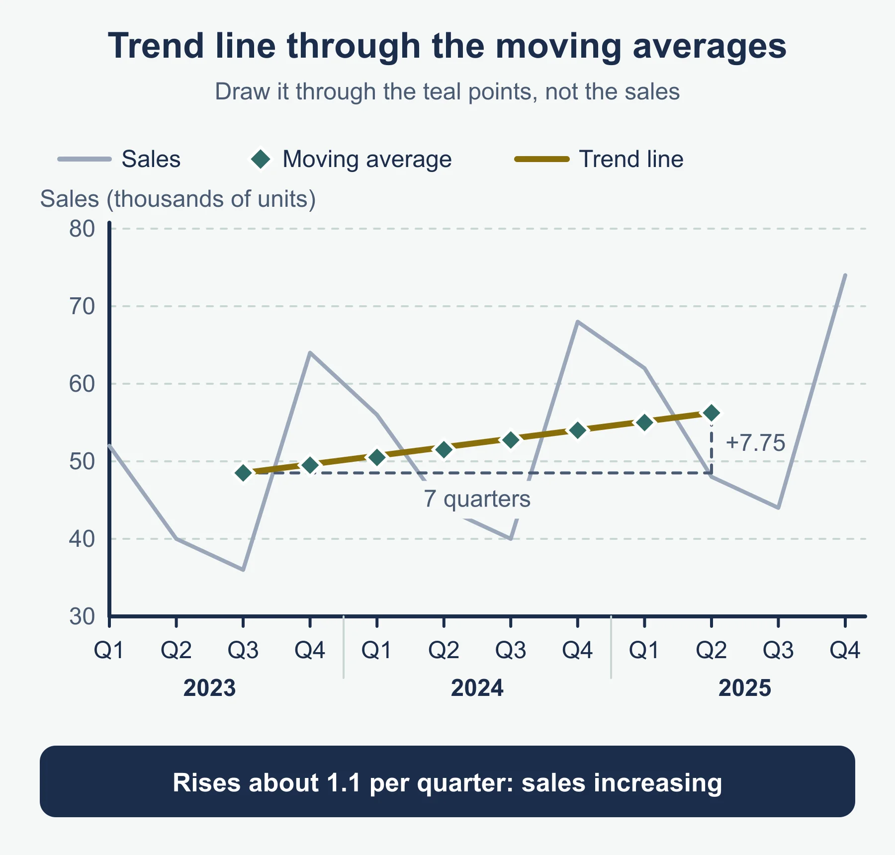
5. Place each average at the middle of its group.
6. If the number of points is even, the middle lies between two time periods, so centre: take the mean of each pair of neighbouring moving averages.

Points	Middle of the first group	Centring needed?	Values lost
Odd (3, 5, 7)	An actual time period	No	(n − 1)/2 at each end
Even (4, 12)	Between two periods	Yes	n/2 at each end after centring

Count check: a series of N values gives N − n + 1 moving averages with n points. For 4 points and centring that is N − 3, then one fewer after centring, so N − 4. With 12 values you get 9 four-point averages and 8 centred ones.

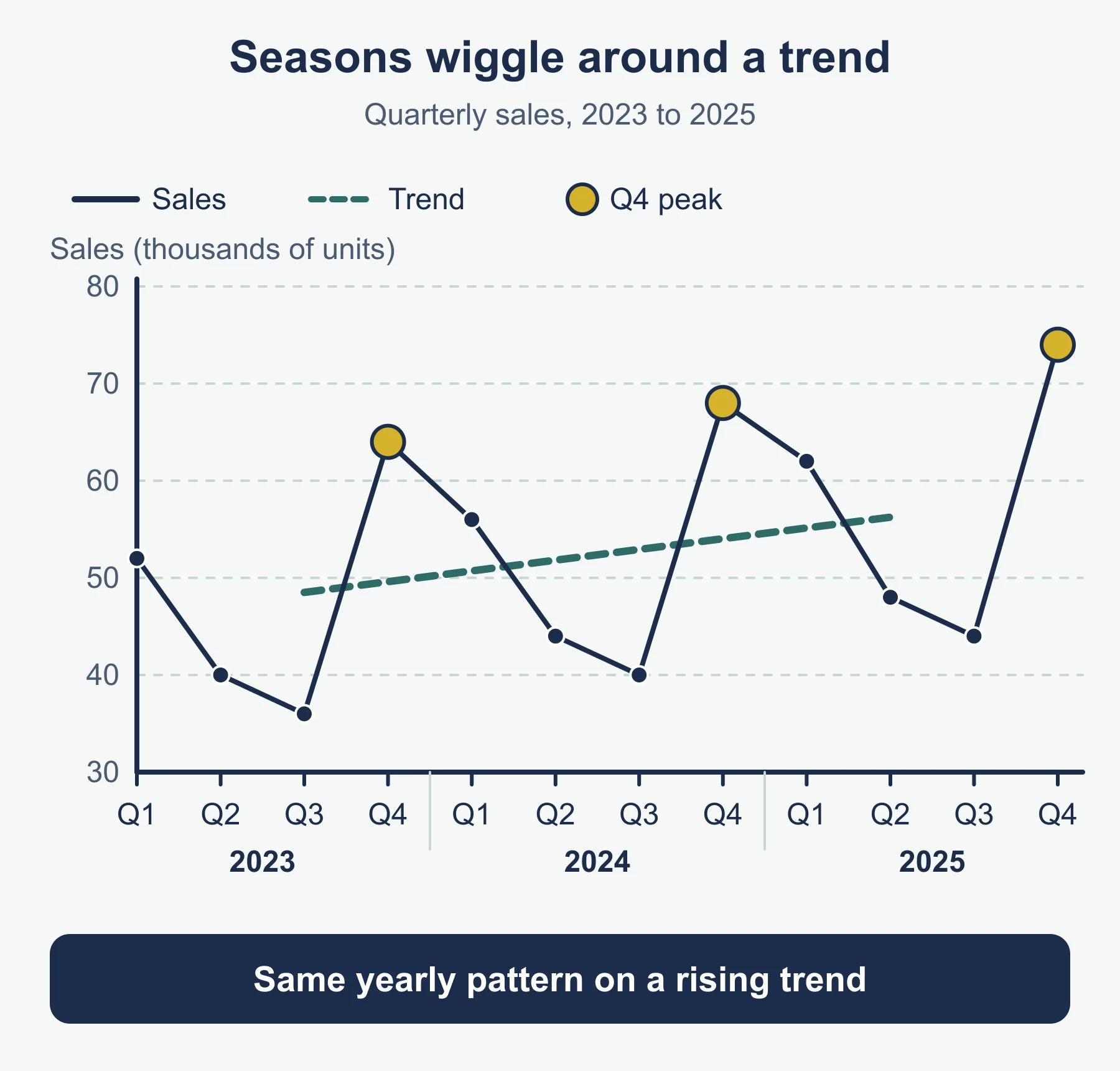
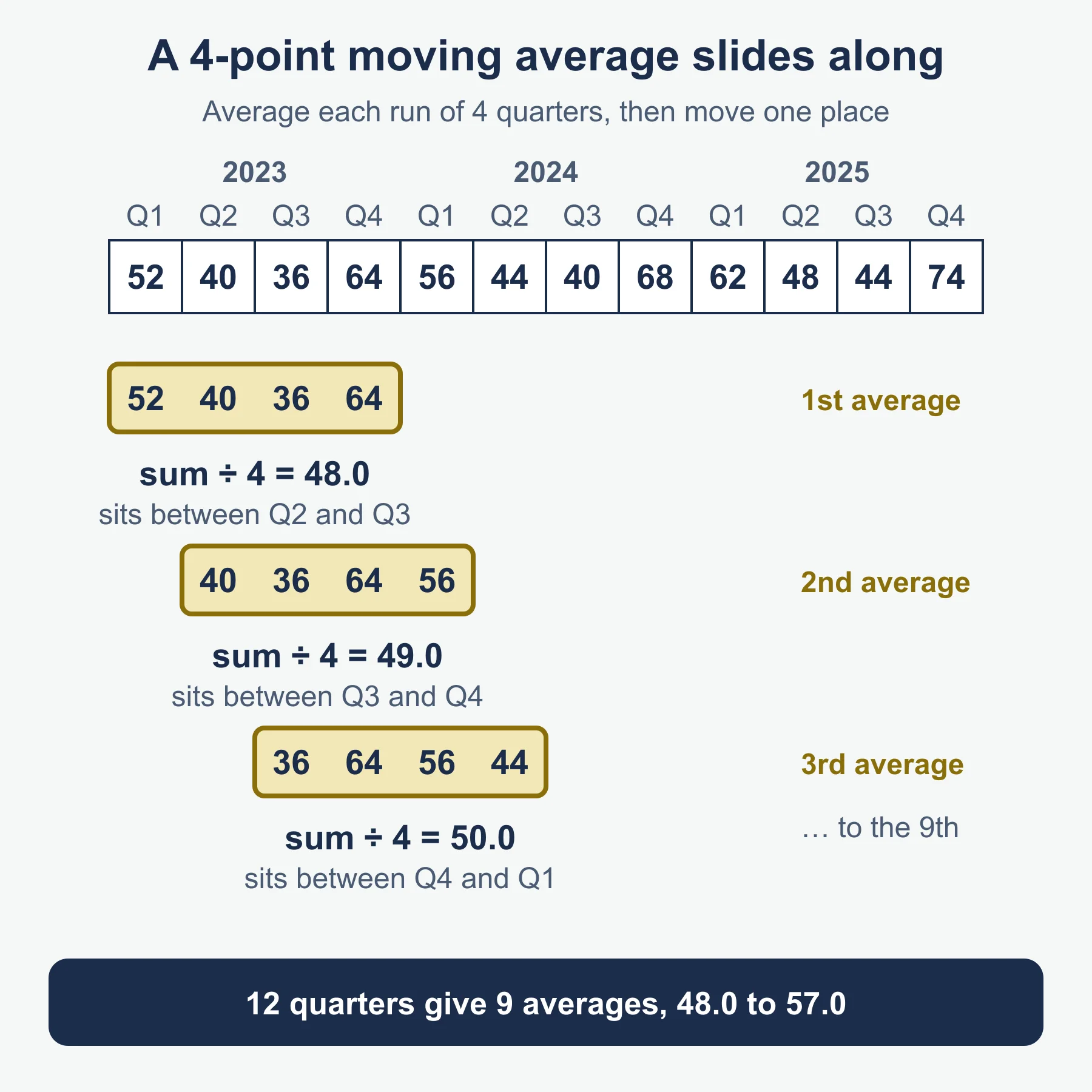
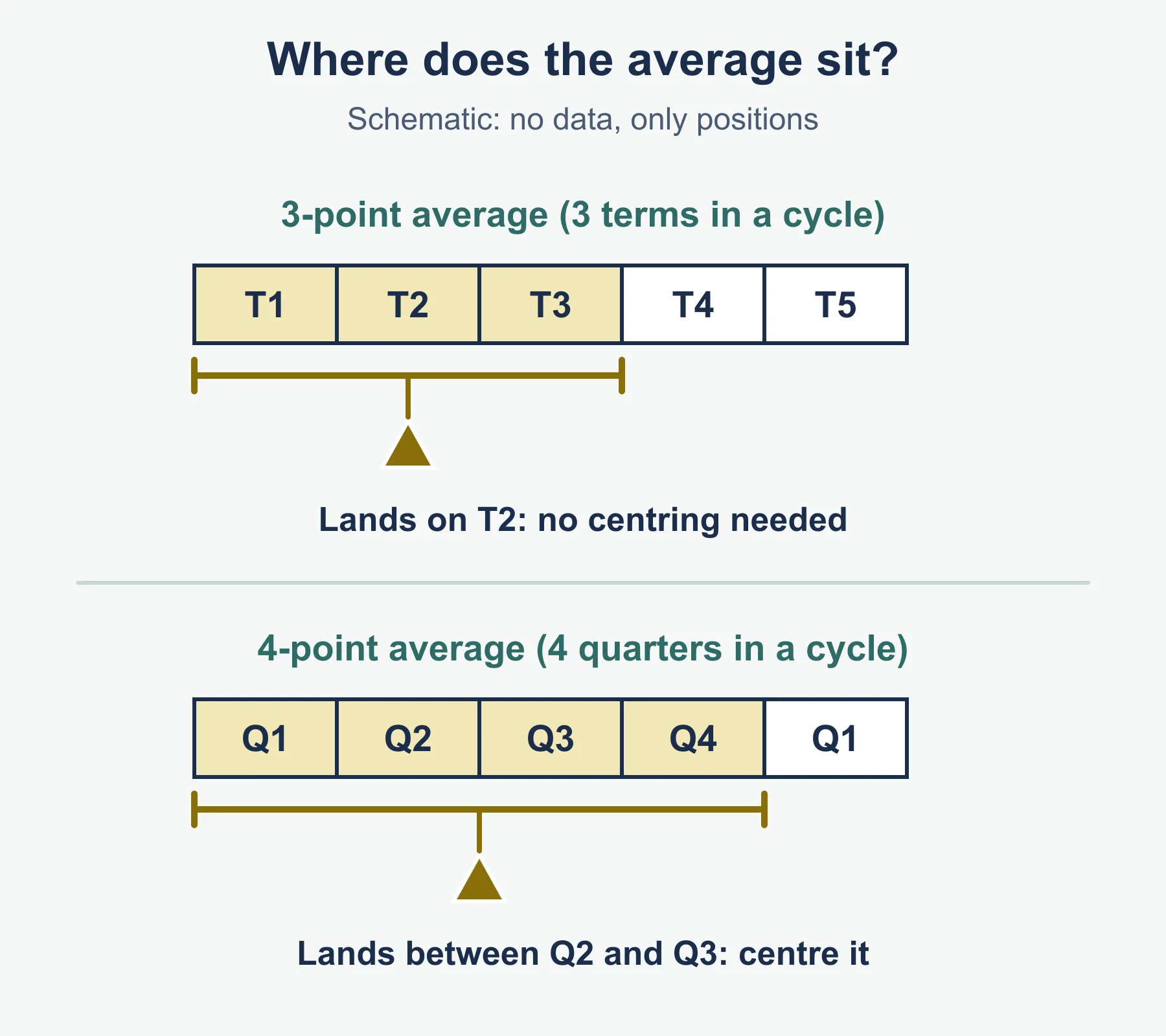
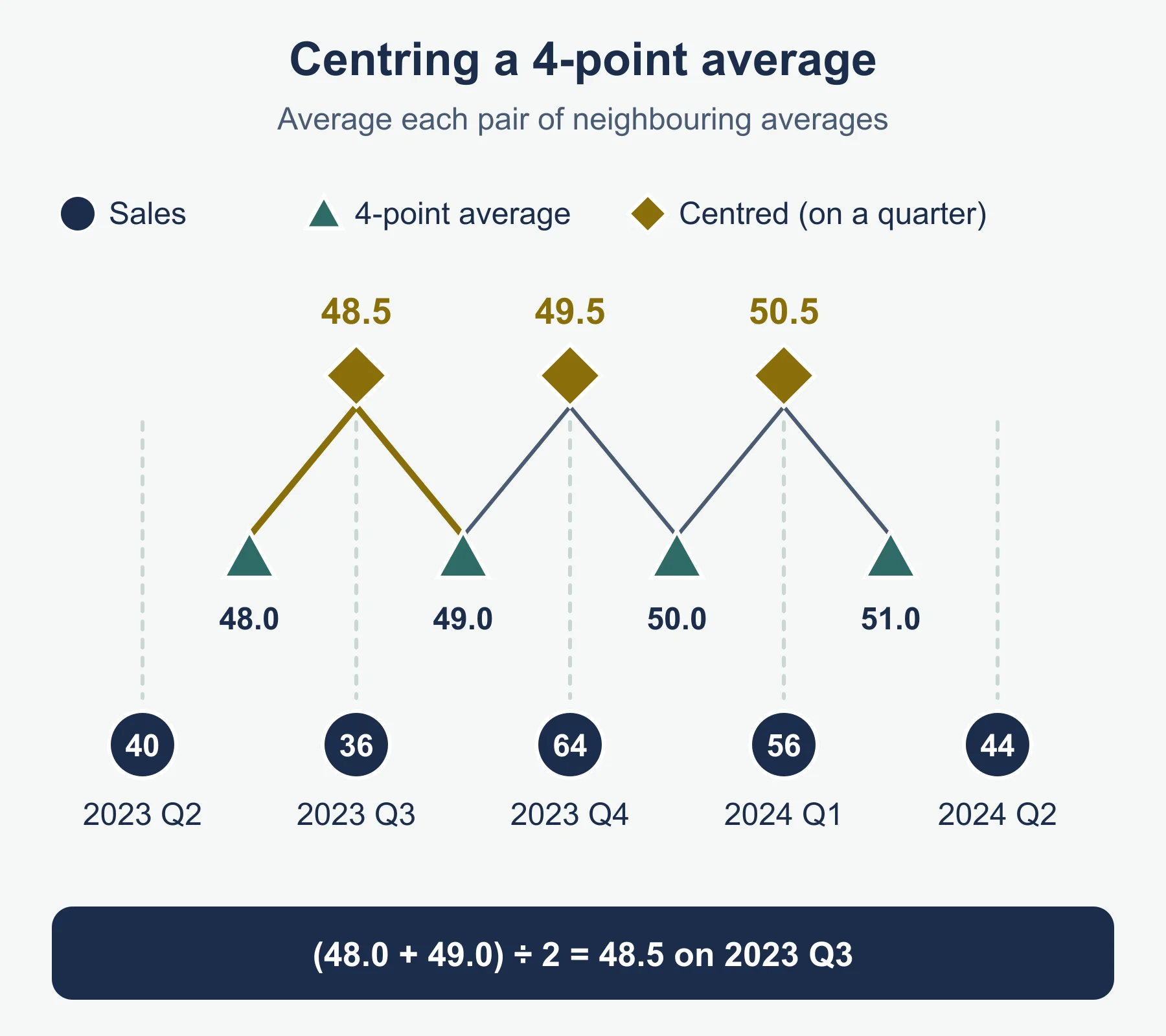
3. Worked reminder: centred 4-point averages

A ferry company records passengers (hundreds) each quarter for three years.

	Q1	Q2	Q3	Q4
Year 1	88	64	52	96
Year 2	82	60	47	90
Year 3	76	55	43	83

Four-point moving averages (each sits between two quarters):

75.0, 73.5, 72.5, 71.25, 69.75, 68.25, 67.0, 66.0, 64.25

Centred (mean of neighbouring pairs), with the quarter each belongs to, and the difference passengers − centred average:

Quarter	Passengers	Centred average	Difference
Year 1 Q3	52	74.25	−22.25
Year 1 Q4	96	73.0	+23.0
Year 2 Q1	82	71.875	+10.125
Year 2 Q2	60	70.5	−10.5
Year 2 Q3	47	69.0	−22.0
Year 2 Q4	90	67.625	+22.375
Year 3 Q1	76	66.5	+9.5
Year 3 Q2	55	65.125	−10.125

The first centred average belongs to the third quarter of the data, and the last to the third-from-last (Year 3 Q2), because a four-point average needs two periods either side. The centred averages fall steadily, so the trend is downward, about 1.3 hundred per quarter.

4. Worked reminder: odd cycle, no centring

Takings (in tens of rupees) at a stall on school days, over three weeks:

	Mon	Tue	Wed	Thu	Fri
Week 1	41	38	35	44	52
Week 2	43	40	37	46	54
Week 3	45	42	39	48	57

The cycle is five days, so use 5-point averages. The first is (41 + 38 + 35 + 44 + 52) ÷ 5 = 42.0 and it belongs to Wednesday of Week 1. The averages then rise by about 0.4 each day (42.0, 42.4, 42.8, 43.2 and so on), so the trend is gently upward. No centring is needed.

5. Drawing and describing the trend

• A time series graph has time along the horizontal axis and the recorded value up the vertical axis. Plot one point per period, join the points with straight lines in time order, and label both axes with units.
• Plot the original series and mark the moving averages on the same graph, each at the time of its middle value.
• Draw the trend line by eye through the moving averages, with roughly equal numbers of points either side. It should follow the moving averages, not the raw data.
• Describe the trend with a direction and a size: “falling by about 1.3 hundred passengers per quarter”.
• To get a gradient, read two well-separated points on the line and divide the change in value by the change in time.

6. Seasonal component: method in steps

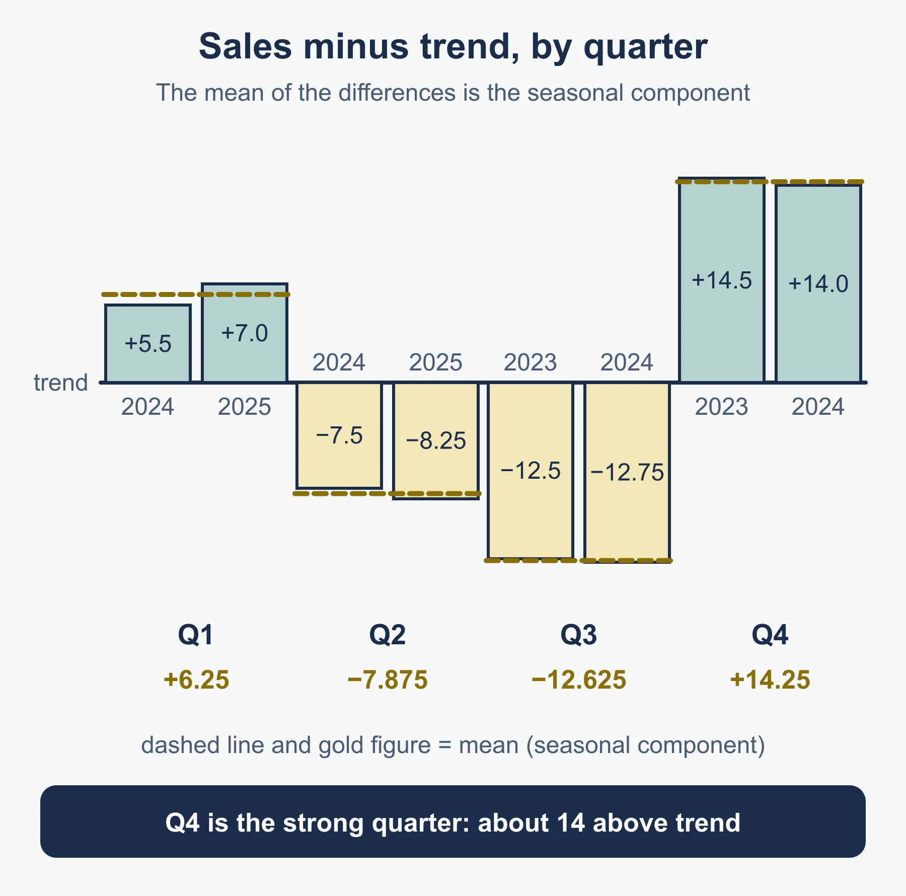
1. Calculate the difference for every period that has a centred or moving average: actual value − moving average.
2. Group the differences by season (all the Q1 differences together, and so on).
3. Take the mean of each group. That mean is the seasonal component for that season.
4. Sense-check: positive for seasons that peak, negative for troughs, and the components should add to roughly zero.

Ferry data from section 3:

Season	Differences	Seasonal component
Q1	+10.125, +9.5	+9.8125, about +9.8
Q2	−10.5, −10.125	−10.3125, about −10.3
Q3	−22.25, −22.0	−22.125, about −22.1
Q4	+23.0, +22.375	+22.6875, about +22.7

Total of the four components: 0.0625, close to zero, which is what you expect. Interpretation: in a typical third quarter the ferry carries about 2 210 fewer passengers than the trend.

Components from a graph and trend line. If the data are plotted with a trend line drawn, read the trend value at each season’s time from the line, then work out plotted value − trend value as a vertical gap (above the line is positive, below is negative). Group the gaps by season and average them exactly as above. For example, if three Q2 points lie 9, 10 and 11 below the line, the Q2 component is −10. Readings from a graph are approximate, so state the values you read.

7. Prediction using trend and seasonal component

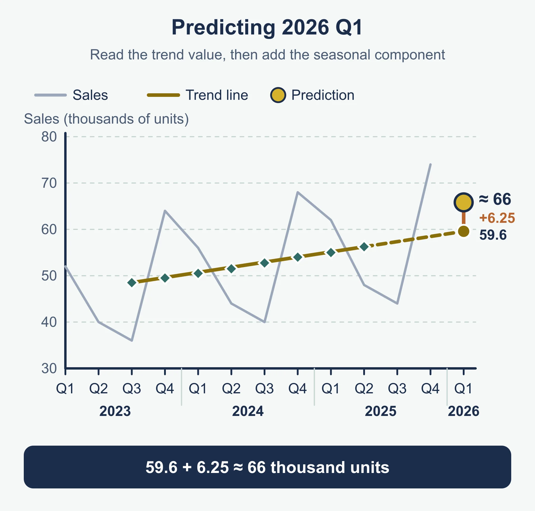
Predicted value = trend value + seasonal component.

Ferry example, Year 4 Q1. The line through the first and last centred averages falls from 74.25 to 65.125 over 7 quarters, which is a change of −1.30 per quarter. Year 4 Q1 is 3 quarters after Year 3 Q2, so the trend value is 65.125 − 3 × 1.30 = 61.2. Add the Q1 component: 61.2 + 9.8 = 71.0 hundred passengers.

Limitations to quote:

• It assumes the trend carries on in the same straight line, and this is shakier the further ahead you predict.
• It assumes each season keeps the same size of effect.
• A trend line drawn by eye gives slightly different answers for different people.
• One-off events (a strike, a new route, bad weather) are not in the model.

8. Must-know distinctions

• Moving average vs mean of all values: the moving average changes along the series; it follows the trend.
• Centred vs uncentred: centring only matters for an even number of points.
• Trend vs seasonal variation: trend is the slow direction; seasonal variation is the repeating swing around it.
• Seasonal component vs difference: a difference belongs to one period; the component is the mean of the differences for that season.

Quick self-test

1. How many points should each moving average have for data collected for every month of the year?
2. A series has 20 values. How many four-point moving averages are there, and how many after centring?
3. For the series 30, 18, 22, 34, 32, 20, 24, 36 (quarterly, starting at Q1), calculate the four-point moving averages.
4. Centre your answers to question 3 and state which values of the series they line up with.
5. Calculate the three-point moving averages of 12, 15, 9, 14, 18, 12.
6. Why does a five-point moving average not need centring?
7. Three seasonal components are +5.2, −3.1 and −6.0, and there is one more season. What value would you expect for it?
8. Sales in one period are 120 and the centred moving average is 100. What is the difference, and what does a positive difference mean?
9. The trend value for a future period is 53.5 and the seasonal component is −6.5. Give the prediction.
10. Give two reasons why a prediction several periods ahead may be unreliable.

Answers

2. 17 four-point averages (20 − 4 + 1); 16 after centring.
3. 26.0, 26.5, 27.0, 27.5, 28.0.
4. 26.25, 26.75, 27.25, 27.75, lining up with the third to sixth values: 22, 34, 32 and 20.
5. 12.0, 12.7, 13.7, 14.7 (to 1 d.p.; the exact values are 12, 12 2/3, 13 2/3 and 14 2/3).
6. The middle of five consecutive values is the third value, which is an actual time period.
7. About +3.9, so that the four components total roughly zero.
8. 120 − 100 = +20; the period is above the trend.
9. 53.5 − 6.5 = 47.0.
10. Any two of: the trend may not continue in a straight line; the seasonal pattern may change; one-off events are not allowed for; the trend line was drawn by eye.

Where marks are usually lost

• Choosing the number of points from the number of values rather than from the length of the cycle.
• Leaving four-point averages uncentred, so they are plotted between two periods.
• Attaching the first centred average to the first period instead of the third.
• Working out moving average − actual, which reverses every sign.
• Drawing the trend line through the raw data instead of through the moving averages.
• Adding the seasonal component to the last actual value instead of to a trend value.
• Rounding moving averages early, then carrying the rounding into the seasonal components.
• Giving a prediction with no mention of the trend value used, so a slip cannot be followed.
• Writing a limitation that is too vague, such as “it might be wrong”, instead of naming an assumption.

Frequently asked questions

Does a “season” in time series have to be a season of the year? No. A season is any period in a repeating cycle, such as a quarter, a day of the week or a month.

How many moving averages does a series give? A series of N values gives N − n + 1 moving averages with n points. For 4 points that is N − 3, and one fewer after centring, so 12 quarterly values give 9 four-point averages and 8 centred ones.

Why does a five-point moving average not need centring? The middle of five consecutive values is the third value, which is an actual time period. Only moving averages with an even number of points need centring.

How can you check your seasonal components? Components should be positive for seasons that peak and negative for troughs, and together they should add to roughly zero.

Which syllabus sections do these time series notes cover? They cover sections 10.1 (trend) and 10.2 (seasonal variation) of Cambridge O Level Statistics 4040 for examination in 2025, 2026 and 2027, and topic 12 of Cambridge IGCSE Statistics 0479 for 2027.

Official syllabus

Cambridge O Level Statistics 4040, syllabus for examination in 2025, 2026 and 2027, published by Cambridge University Press & Assessment: topic 10, Time series, sections 10.1 and 10.2. For the IGCSE content: Cambridge IGCSE Statistics 0479, syllabus for 2027, topic 12, Time series.