IB DP Business Management: Sales forecasting (HL only) – Revision Notes

These notes condense section 4.3, Sales forecasting (HL only), from Unit 4 of the IB Business management guide, first assessment 2024. For full explanations and worked examples, read the study guide. The guide lists one content point here, the benefits and limitations of sales forecasting (AO3), and lists simple linear regression (HL only) in its toolkit.

Links: course hub, printable checklist, practice questions, Unit 4 overview, and the free diagnostics.

Key definitions

Term	Meaning
Sales forecast	A prediction of future sales, in units, revenue or both. The guide does not define it, so this is a working definition.
Trend	The general direction of sales over time, such as steady growth or decline.
Scatter diagram	A graph of paired data, here time (x) against sales (y).
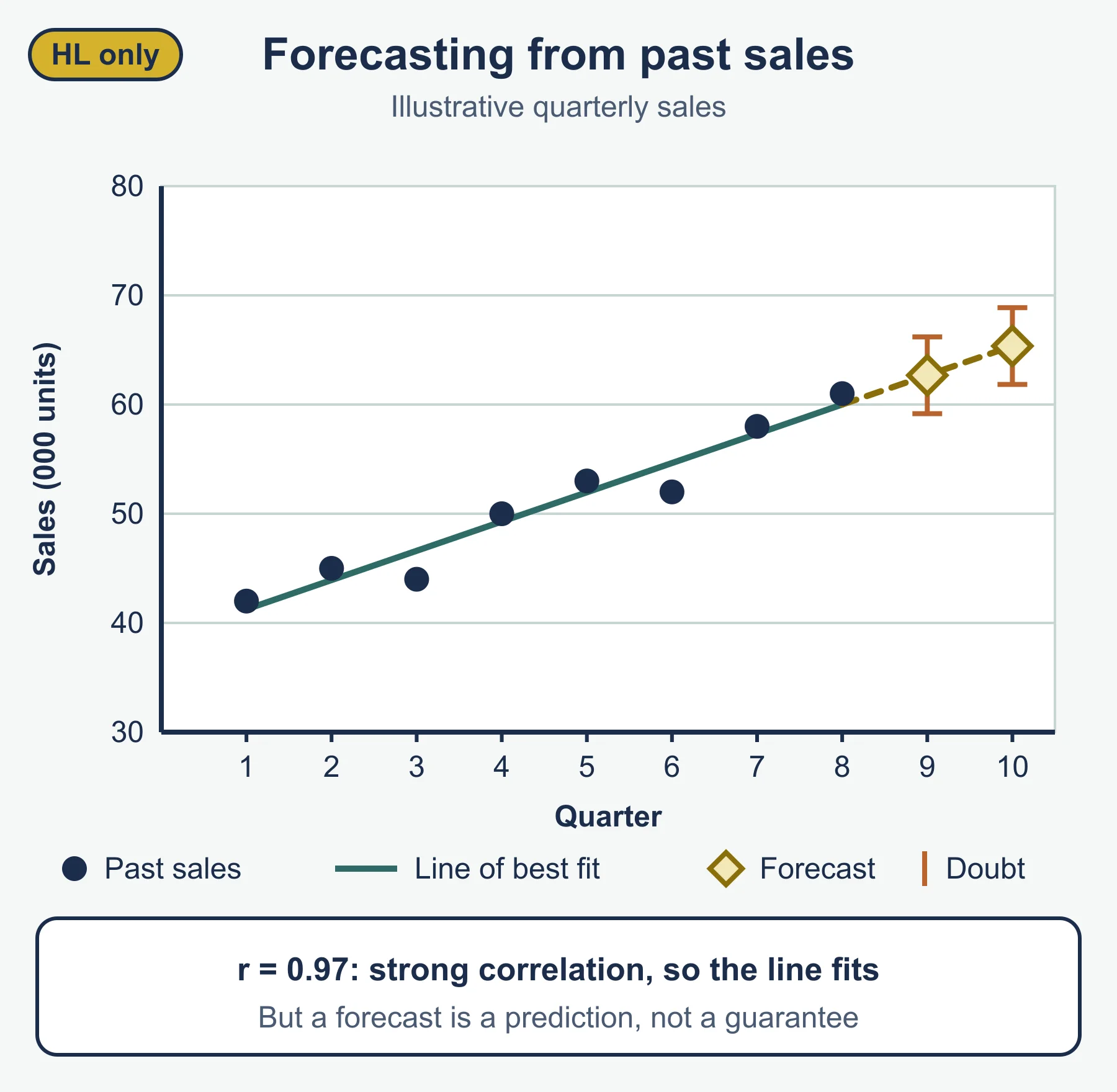
Line of best fit	The straight line that follows the points most closely.
Correlation	How closely points follow a straight line, positive or negative.
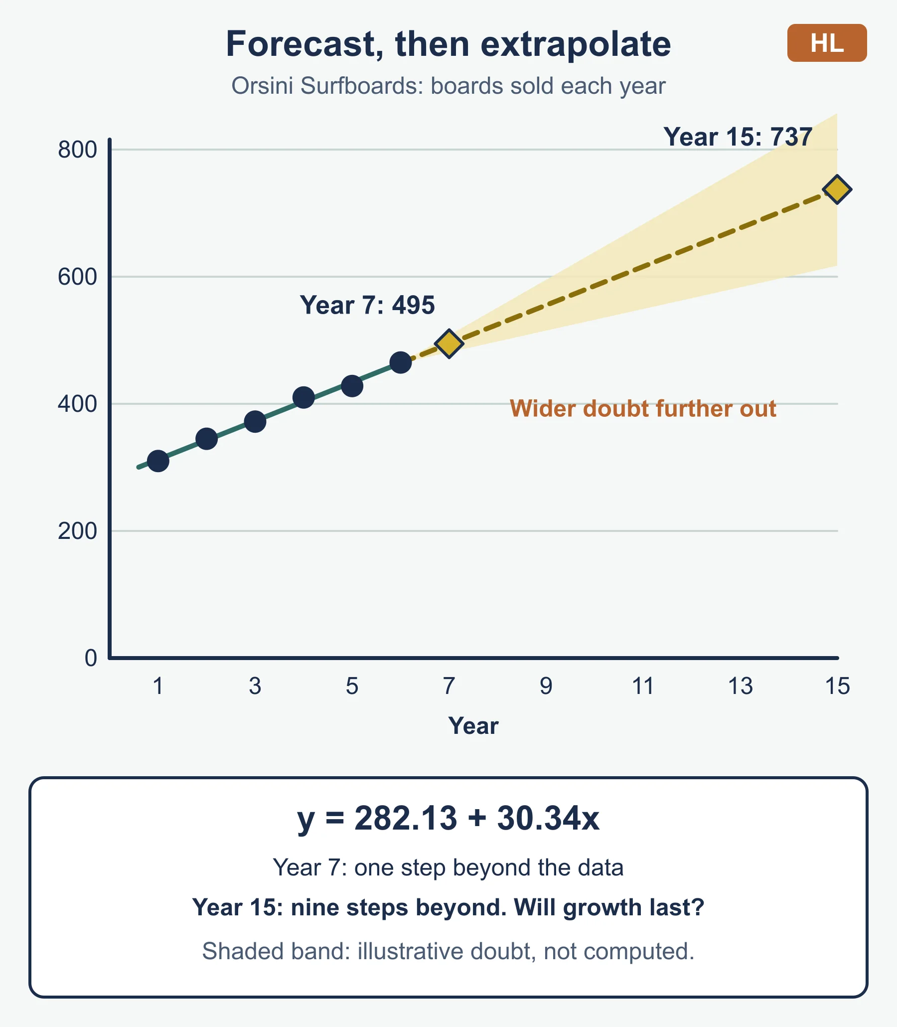
Extrapolation	Extending the line beyond the data to predict a value.
Interpolation	Reading a value from within the range of the data.

Benefits at a glance

Area	How the forecast helps
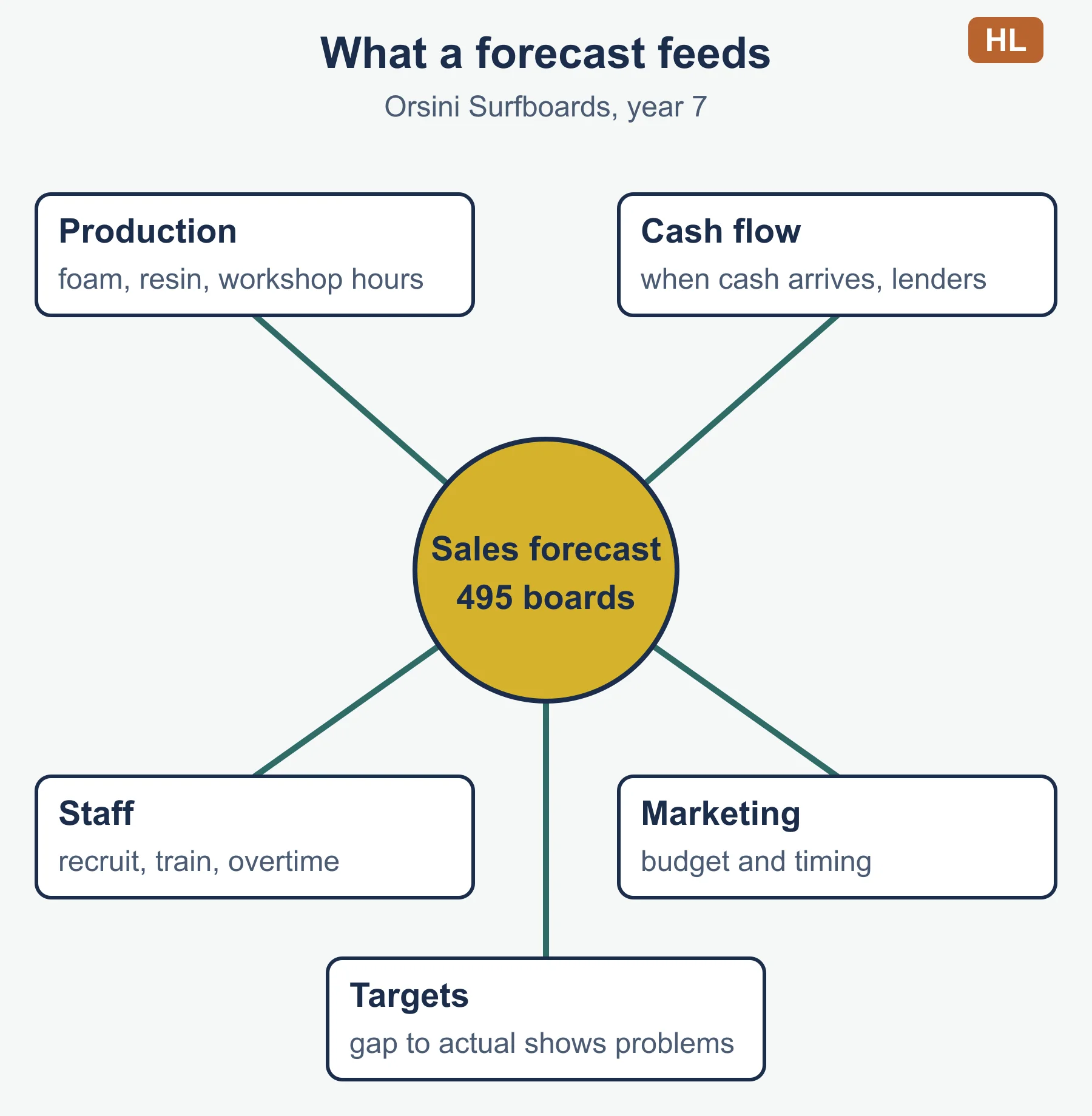
Operations	Plans production, purchasing and stock levels, cutting stockouts and excess stock
Finance	Shapes the cash flow forecast and the case for loans or investment
People	Guides recruitment, training and overtime
Marketing	Sets promotion budgets and tests whether objectives are realistic
Control	Gives targets, and the gap with actual sales shows where to look
Risk	Replaces guesses with evidence, so decisions are easier to defend

Limitations at a glance

Limitation	Why it matters
Past data	Assumes yesterday’s pattern continues
External change	Competitors, tastes, the economy, technology and regulation move demand
Shocks	One-off events are not in any data set
Time horizon	Longer forecasts carry more error
Thin data	New products or few data points give weak lines
Bias	Optimistic or cautious managers distort figures
Cost and time	Data work uses resources
False confidence	A precise number can hide a wide range of outcomes

Method: simple linear regression (HL only)

The guide gives the headings only (scatter diagrams, line of best fit, correlation/extrapolation). The formulas below are the standard least-squares form.

1. Number the periods x = 1, 2, 3 and so on. Record sales as y.
2. Find the means x̄ and ȳ.
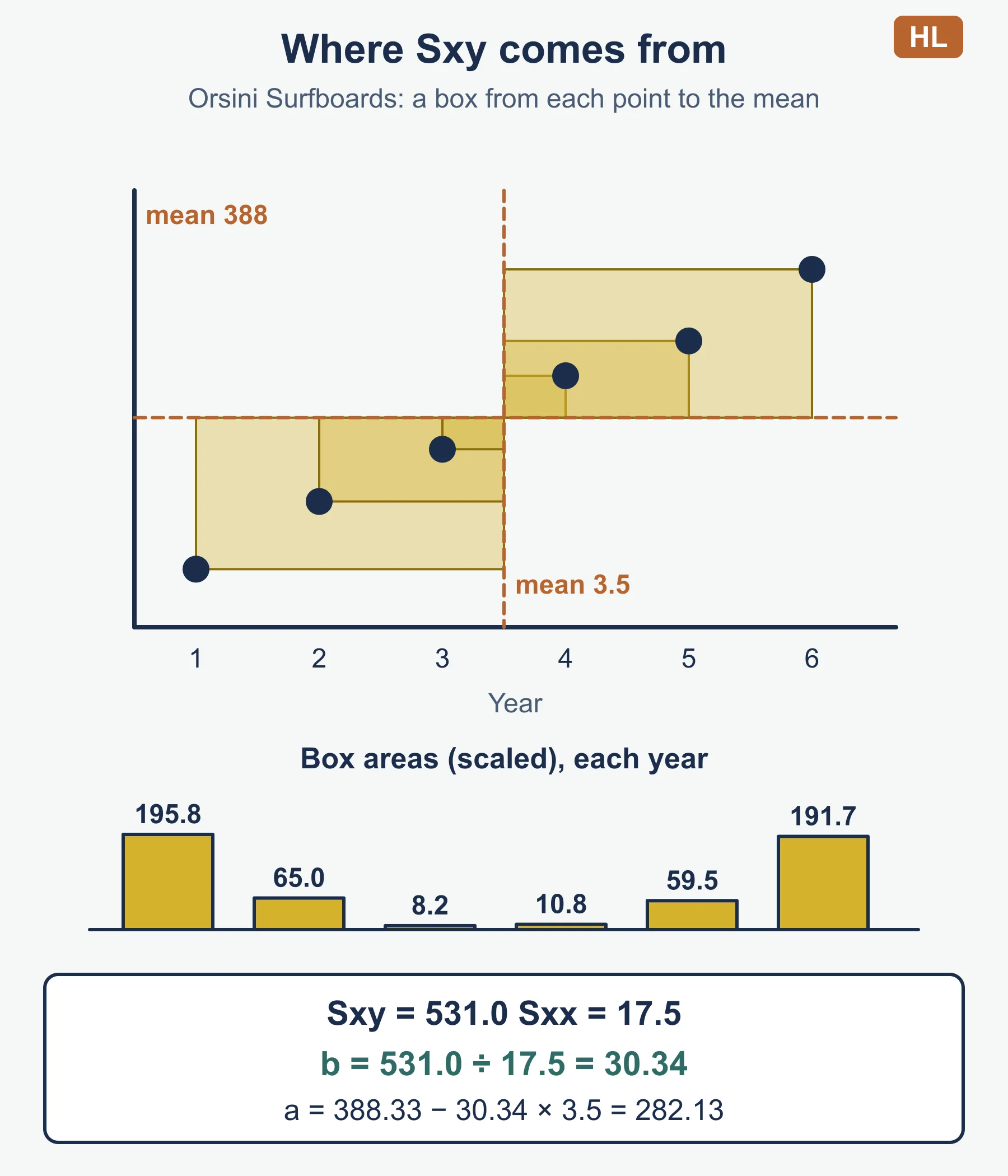
3. Find Sxy = sum of (x − x̄)(y − ȳ) and Sxx = sum of (x − x̄)².
4. Gradient b = Sxy / Sxx. Intercept a = ȳ − b·x̄.
5. Write the line as y = a + bx.
6. Substitute the next period’s x to forecast.
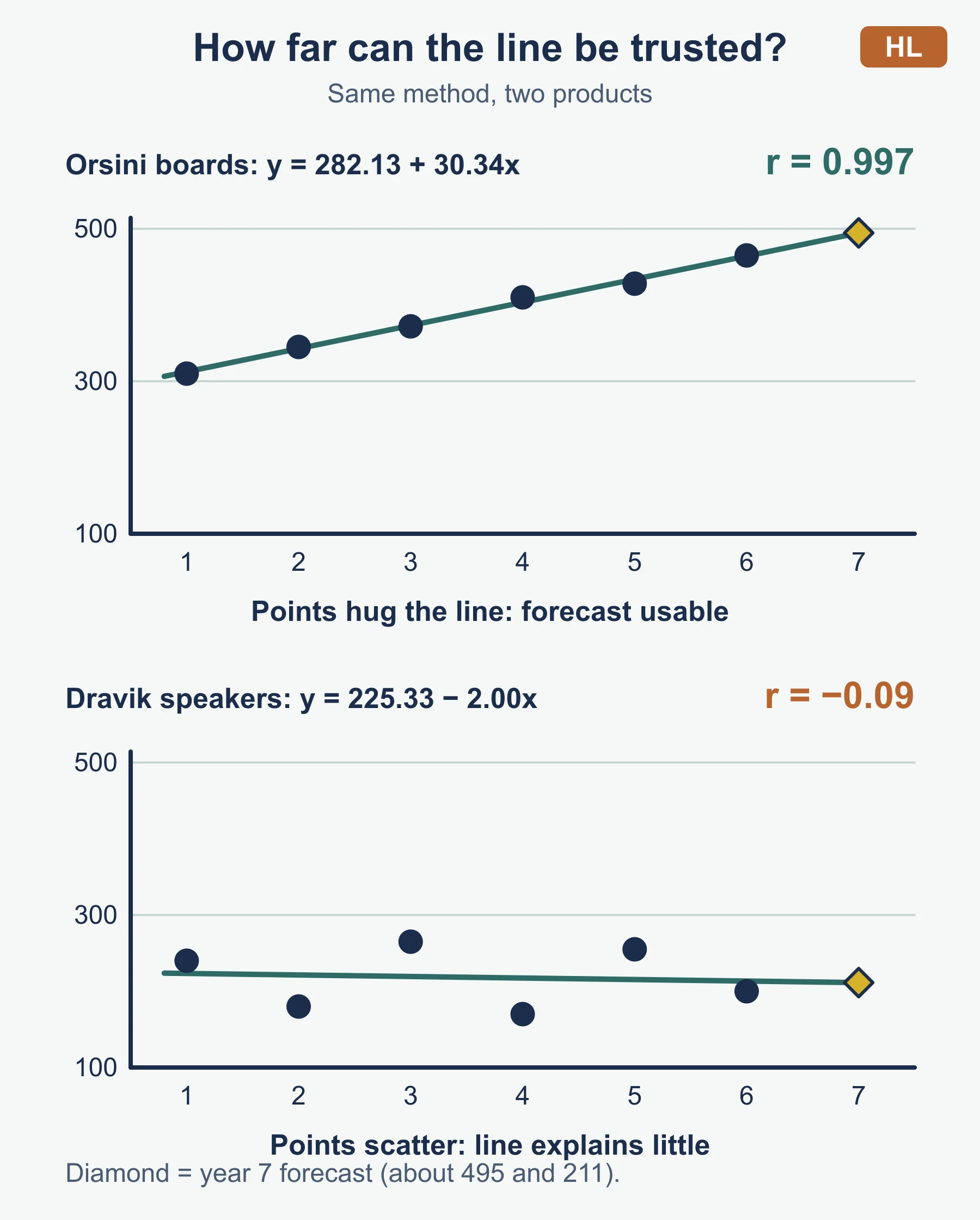
7. Check correlation r (between −1 and +1) before trusting the line.

Item	Standard form
Line of best fit	y = a + bx
Gradient	b = Sxy / Sxx
Intercept	a = ȳ − b·x̄
Correlation coefficient	r = Sxy / √(Sxx × Syy), where Syy is the sum of (y − ȳ)²

Worked reminder

Ulverne Cycles sold 120, 132, 145, 151 and 166 bikes in years 1 to 5.

• x̄ = 3 and ȳ = 142.8.
• Sxy = 111 and Sxx = 10, so b = 11.1.
• a = 142.8 − 11.1 × 3 = 109.5.
• Line: y = 109.5 + 11.1x.
• Year 6 forecast: 109.5 + 11.1 × 6 = 176.1, about 176 bikes.
• r = 0.994, a very strong positive correlation, so a one-year-ahead forecast looks reasonable.

Reading correlation

Value of r	Reading
Close to +1	Strong positive: sales rise steadily with time
Close to −1	Strong negative: sales fall steadily with time
Close to 0	Little or no straight-line relationship: the line is a poor guide

High correlation shows that past points fit a line. It does not show that the future will follow it.

Must-know distinctions

• Sales forecast and cash flow forecast. A sales forecast predicts sales. A cash flow forecast predicts money in and out. The first feeds the second.
• Interpolation and extrapolation. Interpolation stays inside the data range. Extrapolation goes beyond it and is less reliable.
• Strong fit and accurate forecast. A strong fit describes the past. Accuracy depends on whether the future behaves like the past.
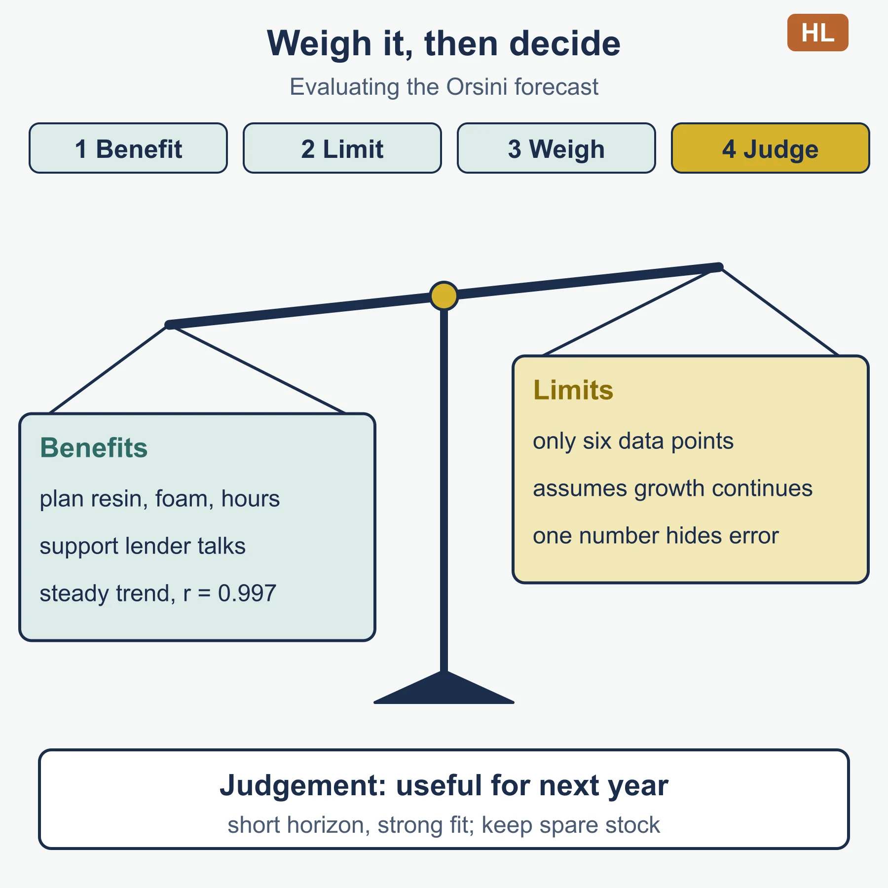
• Benefit and limitation. A benefit is what the forecast lets you do. A limitation is why it may mislead. An evaluation needs both and a judgement.
• Forecast and target. A forecast is a prediction. A target is a goal. Managers sometimes treat one as the other.

Factors that decide the weighing

Factor	Forecast more useful when	Forecast less useful when
Market	Stable, mature demand	Fast-changing tastes or technology
Horizon	Next month or next year	Several years ahead
Cost of error	Stock can be stored or output changed quickly	Goods perish or commitments cannot be undone
Data	Many periods, high correlation	Few periods, correlation near zero
Flexibility	Spare capacity, short supplier lead times	Fixed capacity, long lead times

Linking to other units

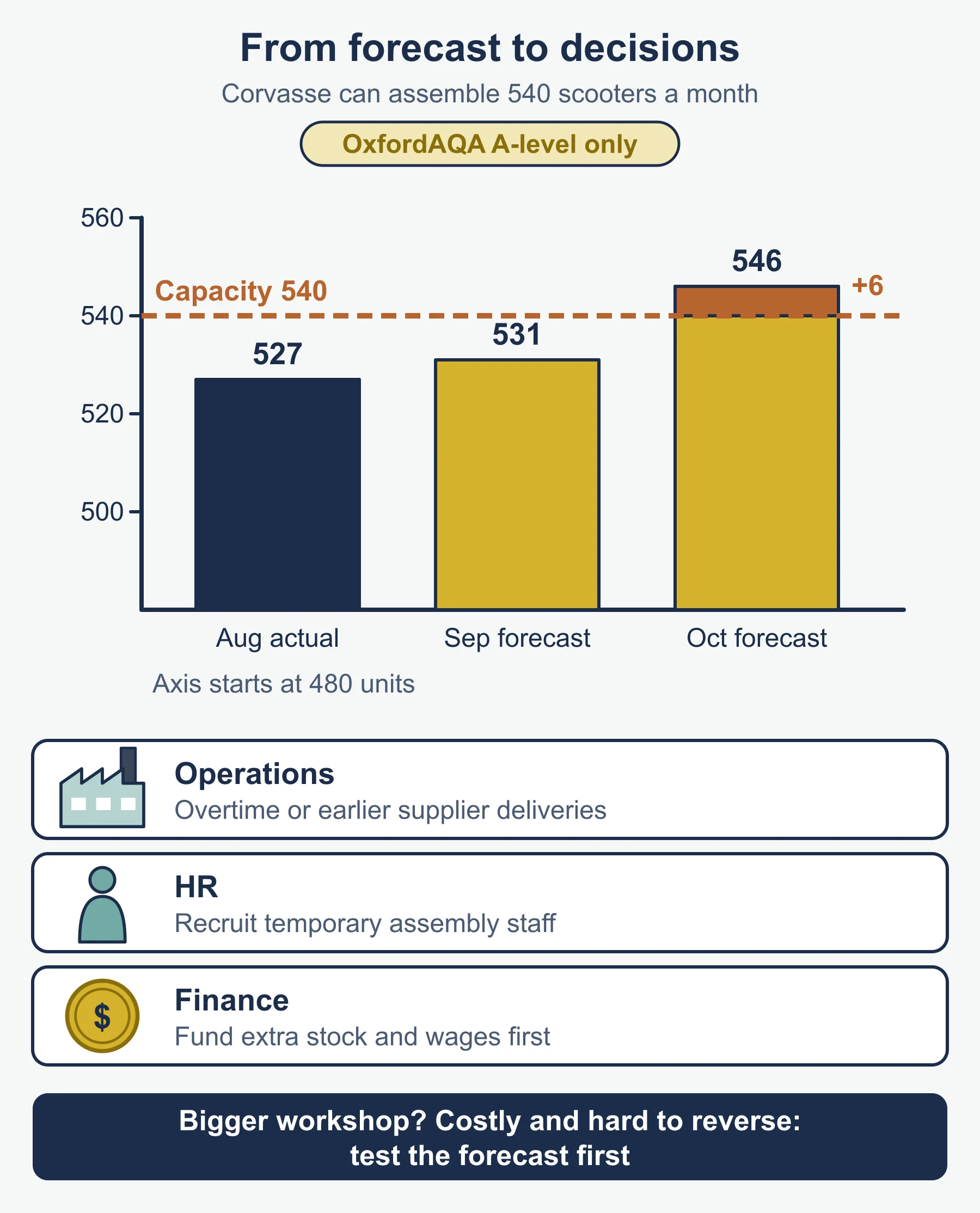
A forecast is an input to other plans, so an error spreads. Too high a forecast leads to surplus stock, tied-up cash and possible price cuts. Too low a forecast leads to stockouts, unmet orders and lost customers. When a case study gives a forecast, test it against capacity, cash and staffing before you praise it.

Percentage check

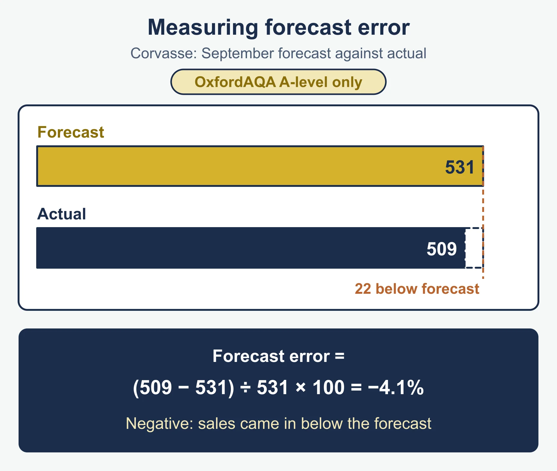
Forecast error is often expressed against the actual figure: (forecast − actual) / actual × 100. If a forecast is 500 and actual is 460, the forecast was 8.7% above actual sales. State which base you used.

How to write an evaluation (AO3)

1. Benefit tied to the business and a decision it supports.
2. Limitation tied to a feature of the case.
3. Weigh using market stability, time horizon, cost of error, data quality and flexibility.
4. Judgement with a reason, such as “useful for next year, less so for five years, because…”.

Quick self-test

1. Define a sales forecast.
2. State two benefits of sales forecasting.
3. State two limitations of sales forecasting.
4. Ulverne’s line is y = 109.5 + 11.1x. Forecast sales for year 6.
5. For Ulverne, r = 0.994. What does this suggest?
6. Use the same line to forecast year 20. Should the owner rely on it?
7. Distinguish between interpolation and extrapolation.
8. A bakery forecast 500 loaves and sold 460. By what percentage did the forecast exceed actual sales? Give the answer to 1 decimal place.
9. What does the command term “evaluate” ask you to do?
10. Explain how a sales forecast links to a cash flow forecast.
11. Give the standard formula for the gradient b.

Answers

1. A prediction of the sales (units, revenue or both) a business expects over a future period.
2. Any two, such as: better production and stock planning; support for the cash flow forecast and borrowing; guides recruitment; helps set marketing budgets; provides targets to check against.
3. Any two, such as: relies on past data; external changes such as competitors or tastes; unexpected events; less reliable further ahead; thin data; bias.
4. 109.5 + 11.1 × 6 = 176.1, so about 176 bikes.
5. A very strong positive correlation. Sales have risen steadily and the points fit the line closely, which supports a short-range forecast.
6. 109.5 + 11.1 × 20 = 331.5, so about 332 bikes. This is far beyond the five years of data, so the owner should not rely on it. The market, competitors or tastes could change.
7. Interpolation reads a value from inside the range of the data. Extrapolation extends the line beyond the data and carries more risk.
8. (500 − 460) / 460 × 100 = 8.7%.
9. Make an appraisal by weighing up strengths and limitations, and reach a reasoned judgement.
10. Expected sales revenue shapes expected cash inflows, and expected volumes shape purchases and wages, which are cash outflows. A wrong sales forecast therefore makes the cash flow forecast wrong too.
11. b = Sxy / Sxx, where Sxy is the sum of (x − x̄)(y − ȳ) and Sxx is the sum of (x − x̄)².

Where marks are usually lost

• Listing benefits and limitations in general terms without linking them to the business in the case.
• Stopping at “it might be wrong” instead of saying what in the case could make it wrong.
• Calling a forecast certain, or calling it useless, with no balance.
• Treating a high correlation as proof of future accuracy.
• Extrapolating a long way from the data and quoting the answer with no warning.
• Mixing up the sales forecast and the cash flow forecast.
• Leaving out the judgement in an “evaluate” or “justify” question.
• Slips in the regression arithmetic, such as using the wrong mean or mixing up the sign of b. Show each step so the working can be followed.

Next steps

Try the practice questions, return to the study guide for any gaps, and tick off the topic on the checklist.

Frequently asked questions

What is the difference between interpolation and extrapolation? Interpolation reads a value from inside the range of the data. Extrapolation extends the line beyond the data to predict a future value, which becomes less reliable the further it goes.

How do you calculate forecast error as a percentage? Forecast error is often expressed against the actual figure: (forecast − actual) ÷ actual × 100. For example, forecasting 500 loaves and selling 460 gives an error of 8.7%.

What is the difference between a sales forecast and a cash flow forecast? A sales forecast predicts sales, in units or revenue. A cash flow forecast predicts money coming in and going out; the sales forecast feeds into it through expected receipts.

How do you find the gradient of a line of best fit? In standard form, the gradient b = Sxy ÷ Sxx, where Sxy is the sum of (x − x̄)(y − ȳ) and Sxx is the sum of (x − x̄)². The intercept is a = ȳ − b·x̄.

Official syllabus

IB Diploma Programme Business management guide, first assessment 2024, published by the International Baccalaureate Organization. Sections used: 4.3 Sales forecasting (HL only), and the business management tools listing for simple linear regression (HL only).