OCR A Level Business: Forecasting (H431) – Revision Notes

These are quick-recall notes on Forecasting from the Business objectives and strategy area of study in the OCR A Level Business (H431) specification, Version 2.1 (January 2026), with final assessment in summer 2027. Full explanations and worked examples are in the forecasting study guide. Test yourself with the practice questions. Wider context: objectives and strategic decisions guide, strategy revision notes and strategy practice set. Links: course hub, checklist and free 10-minute diagnostics.

Nature and purpose

• Forecast: an informed estimate of a future variable (sales, costs, profit, cash flow, demand).
• Purpose: reduce uncertainty; plan output, staffing, stock and finance; set targets; support funding requests; compare actual with expected results.
• Advantages to a business: better planning, early warning, evidence for lenders, a benchmark for control.
• Disadvantages: based on assumptions, can be wrong, costs time and money, risk of false confidence.
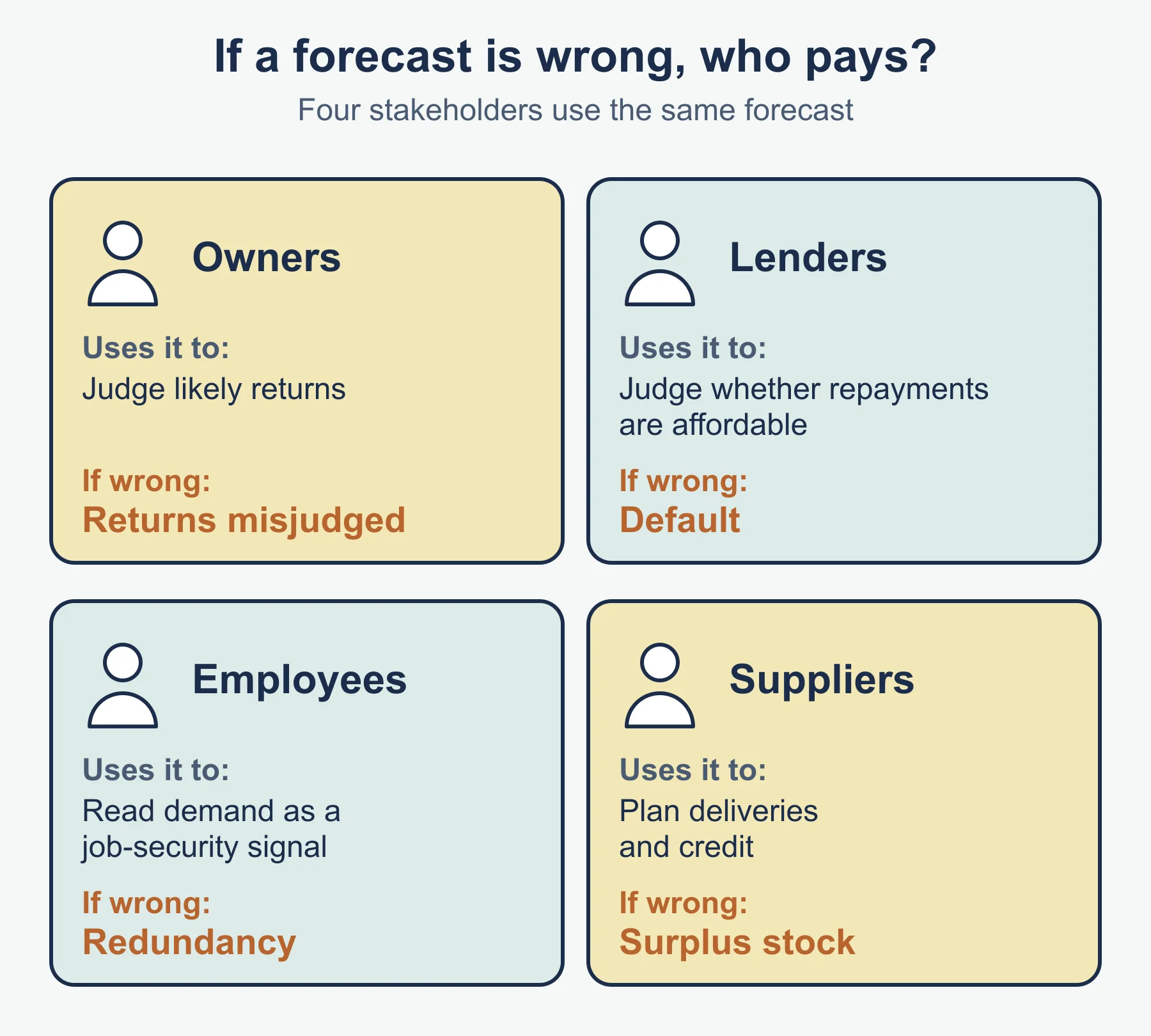
• Stakeholders: owners (returns), lenders (repayment), employees (job security), suppliers (orders and credit). Wrong forecasts hurt each of them in different ways.

Qualitative versus quantitative

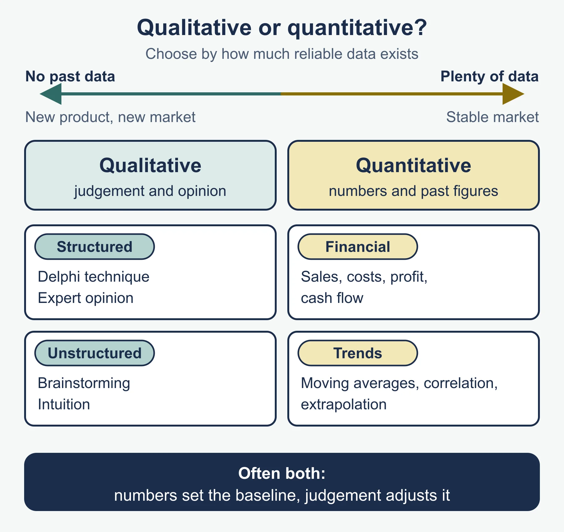
	Qualitative	Quantitative
Based on	Opinion, judgement, experience	Numerical data and calculation
Best when	New product or market, little data	Stable market, good past data
Weakness	Subjective, hard to check	Assumes the past repeats
Cost	Often cheaper and quicker	Data and skills needed

Qualitative methods

Type	Method	How it works	Plus	Minus
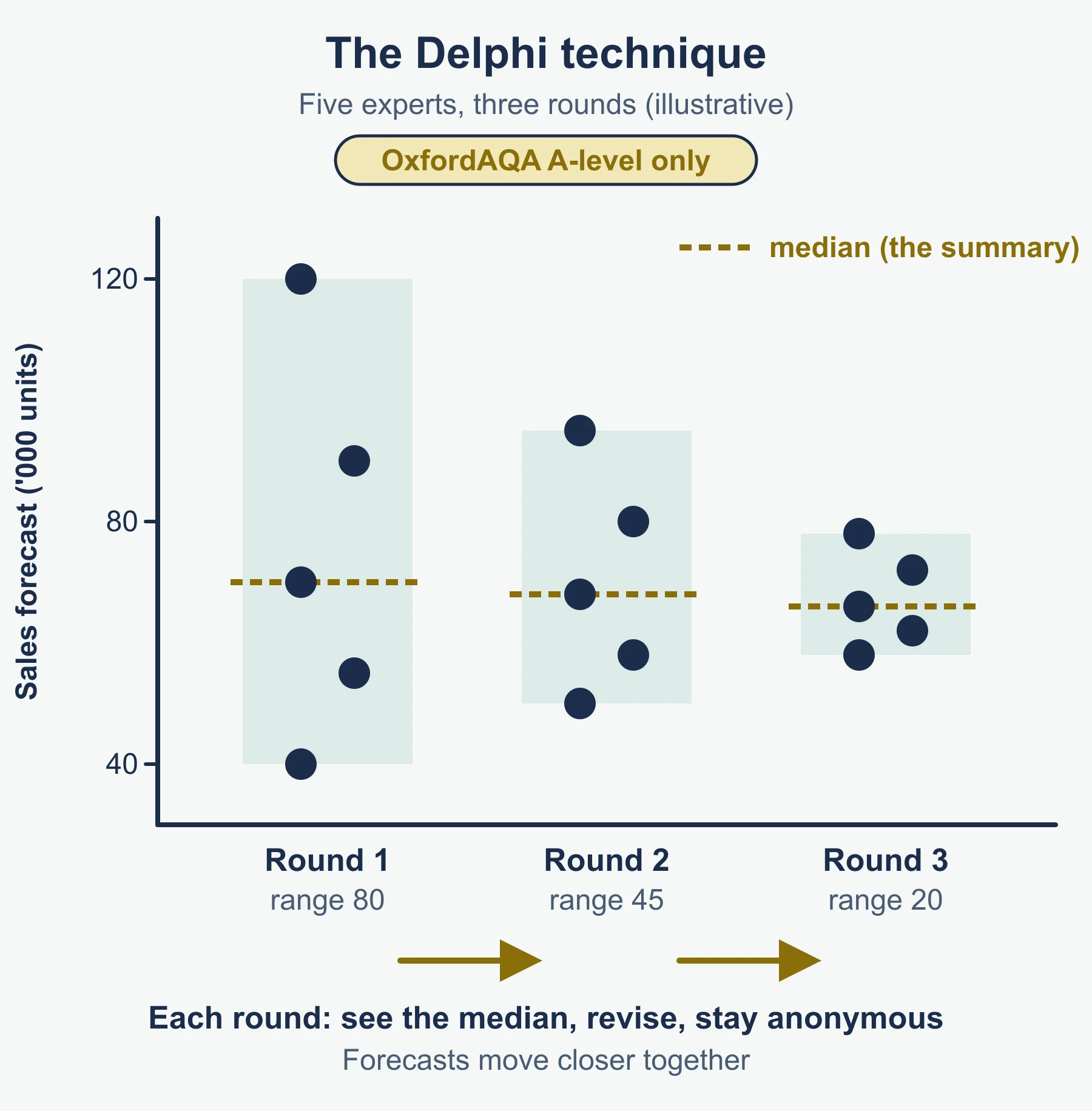
Structured	Delphi technique	Experts give views separately, see an anonymous summary, revise over several rounds	Reduces dominant-voice bias; systematic	Slow, costly; experts may share the same blind spot
Structured	Expert opinion	One or more specialists give a judgement	Quick; specialist knowledge	Depends on one view; may be biased
Unstructured	Brainstorming	Group produces many ideas or predictions without early criticism	Cheap; creative; involves staff	Little rigour; louder voices dominate
Unstructured	Intuition	Manager’s gut feeling from experience	Instant; useful with no data	Subjective; overconfidence

Evaluation hook: the right method depends on the cost of being wrong, the time available and how new the situation is.

Quantitative financial forecasts

Item	Standard form
Sales revenue	units × price
Total costs	fixed costs + variable costs (units × variable cost per unit)
Profit	sales revenue − total costs
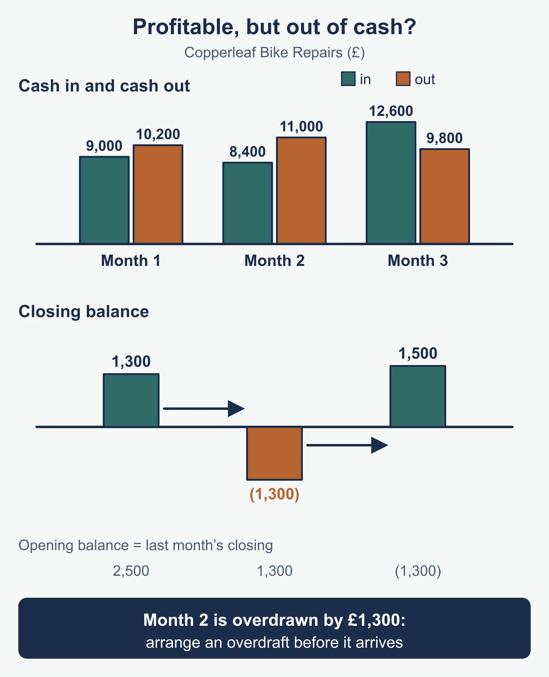
Closing cash	opening cash + cash in − cash out
Next month’s opening cash	this month’s closing cash

Method in steps for a cash-flow forecast

1. Work out sales for each month.
2. Split receipts by credit terms (for example 60% this month, 40% next).
3. List payments in the month they are paid, including one-off items.
4. Net cash flow = cash in − cash out.
5. Closing = opening + net; carry it forward.
6. Interpret: any negative closing balance needs action.

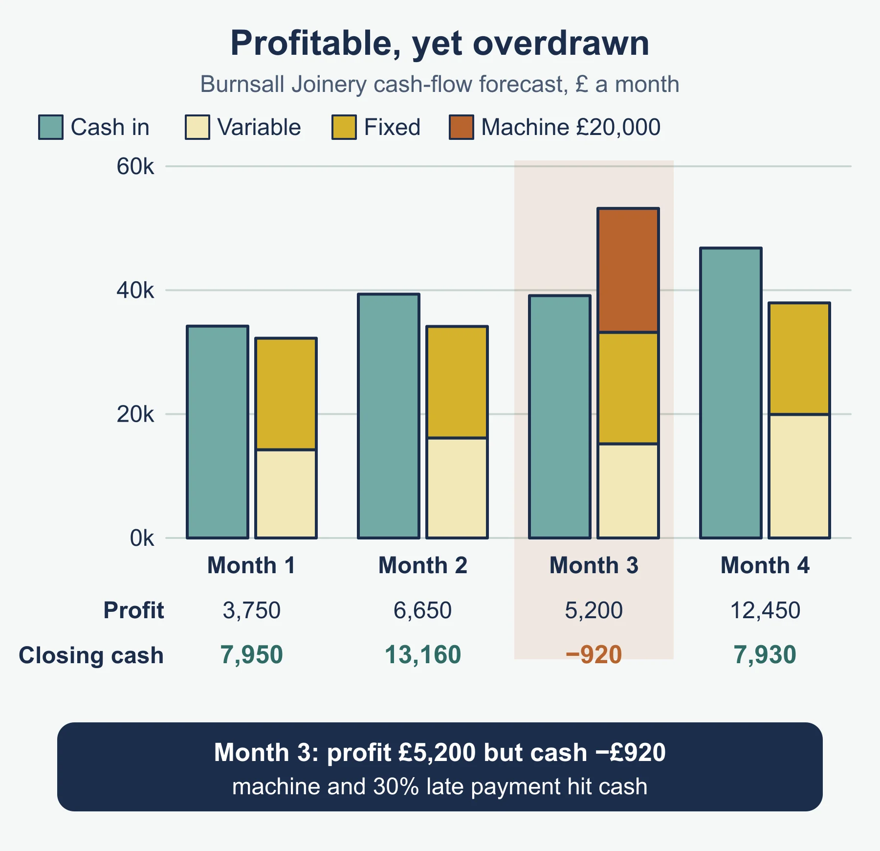
Reminder: profit is not cash. Credit terms, stock purchases and equipment buying shift cash away from profit.

Rushbeck Garden Centre mini-example. A cash forecast shows opening 2,000, receipts 9,000 and payments 11,500. Closing is 2,000 + 9,000 − 11,500 = −500, so the garden centre needs an overdraft or must delay a payment.

Seasonal and cyclical variation

	Seasonal	Cyclical
Length	Within a year	Several years
Cause	Weather, holidays, calendar	Economic or industry cycle
Repeats	Predictably	Irregular in length and size
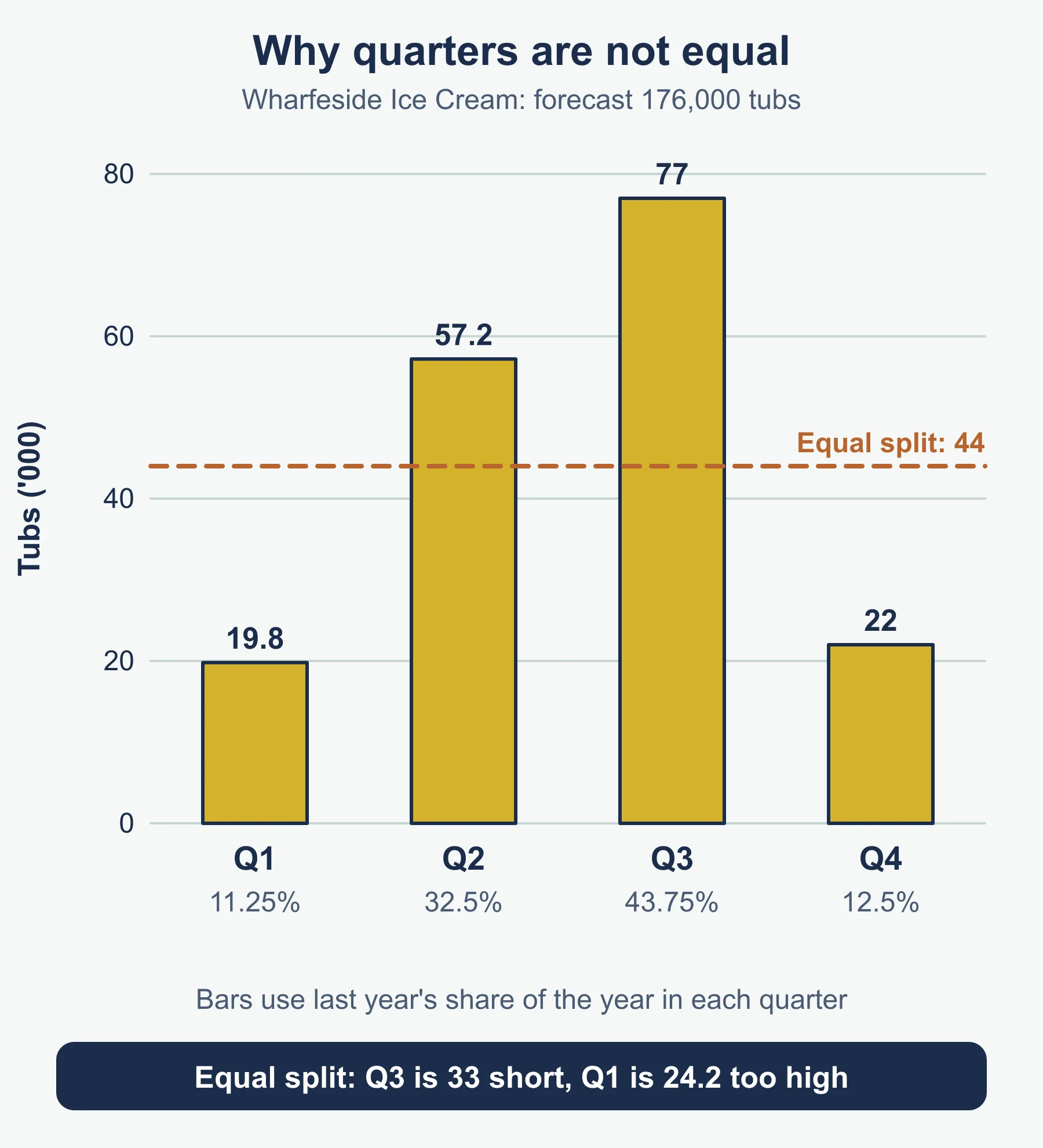
Effect on forecasts	Monthly and quarterly figures differ from the annual average	Boom or slump can be mistaken for permanent change

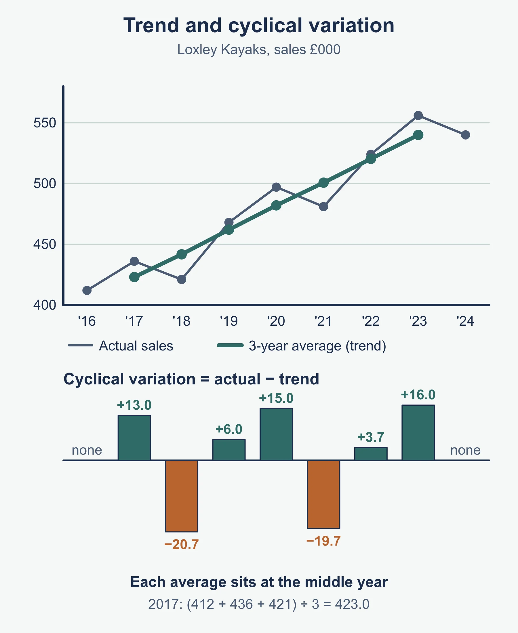
• Trend: the long-run direction, found by a moving average.
• Cyclical variation = actual value − trend value (standard form). Positive: above trend. Negative: below.
• Seasonal illustration: Rushbeck sells 240 plants a year, with shares of 15%, 47.5%, 30% and 7.5% across the quarters. The quarterly forecast is 36, 114, 72 and 18, not 60 each. Using shares like this is a simple illustration, not a method the specification names.
• Impact: ignoring seasonality leads to wrong stock and staffing; ignoring the cycle leads to over-expansion near a peak.

Time series analysis: moving averages (odd number of years)

Three-year moving average for a year = (previous + current + next) ÷ 3, written against the middle year.

Worked reminder: Lindeth Bakery, sales (£000) 2018 to 2024: 88, 92, 97, 95, 103, 108, 112.

Year	Sales	Trend	Cyclical variation
2019	92	92.3	−0.3
2020	97	94.7	+2.3
2021	95	98.3	−3.3
2022	103	102.0	+1.0
2023	108	107.7	+0.3

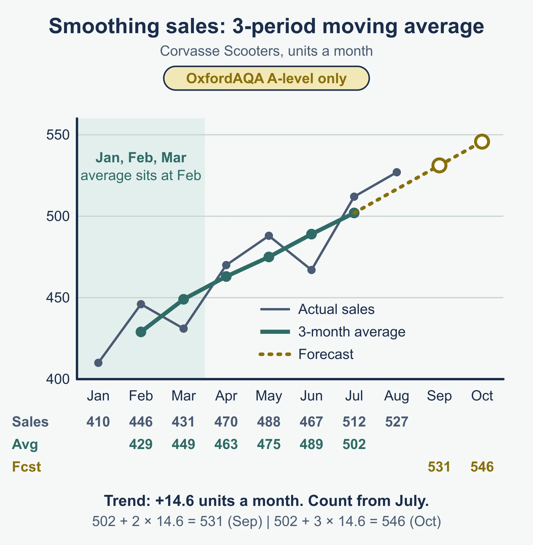
Trend moves from 92.3 to 107.7 over four years, so the average rise is 3.8 a year. Extrapolating: 2024 trend about 111.5, 2025 trend about 115.3. State that this is an estimate.

Method in steps

1. Choose an odd number of years (3 or 5).
2. Add that many consecutive values and divide.
3. Place the result against the middle year.
4. Find the average yearly change in the trend.
5. Extend the trend forward for the forecast.
6. Adjust for known cyclical or seasonal effects, and comment on reliability.

Evaluating time series analysis

• For: objective, cheap, smooths random fluctuation, shows direction.
• Against: assumes the past continues; no value for the latest years; cannot foresee shocks; needs enough reliable data; a longer average reacts more slowly.

Correlation and extrapolation

Pattern on a scatter graph	Correlation
Points rise left to right	Positive
Points fall left to right	Negative
No clear pattern	None
Tight around a line	Strong
Spread widely	Weak

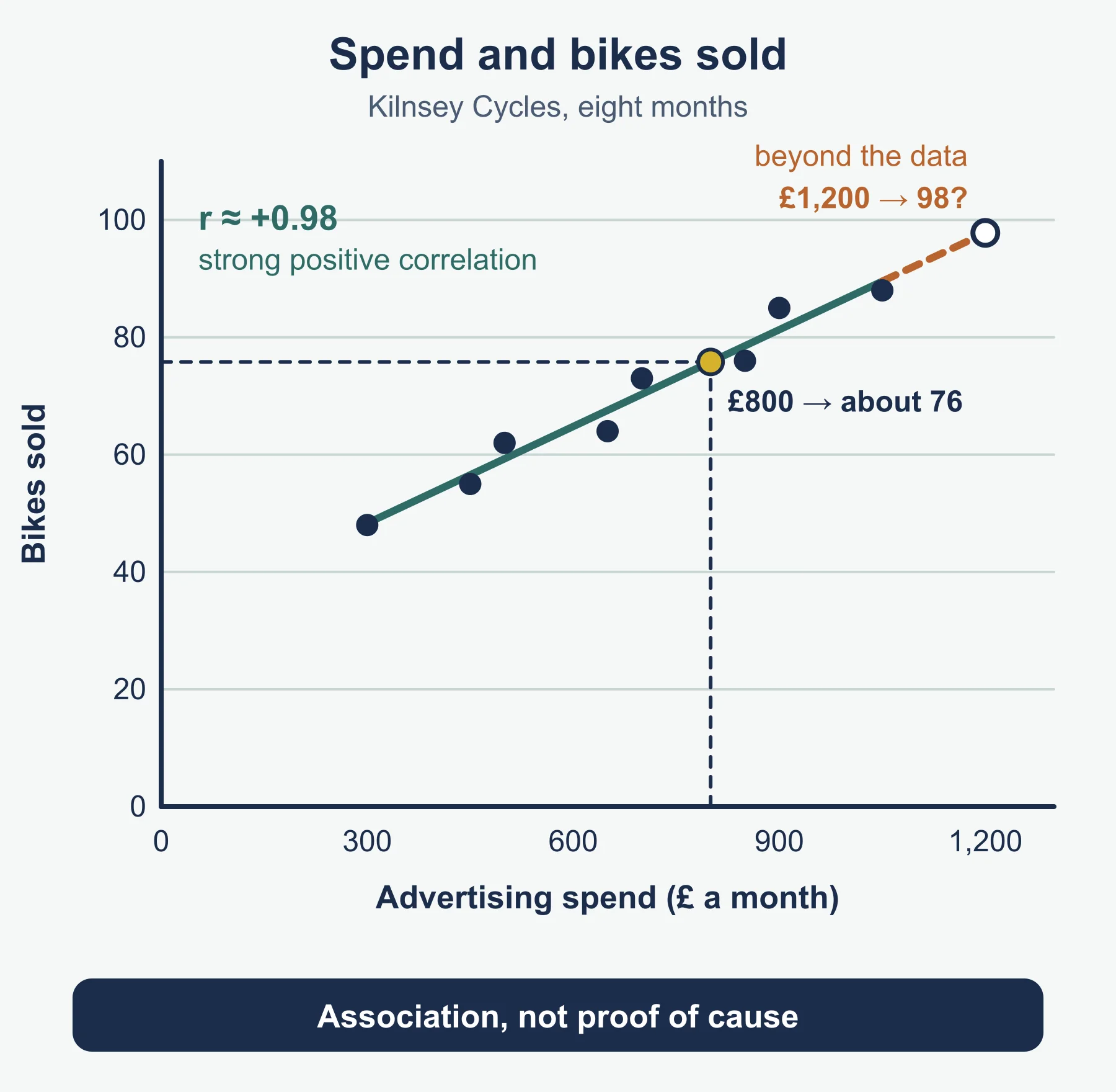
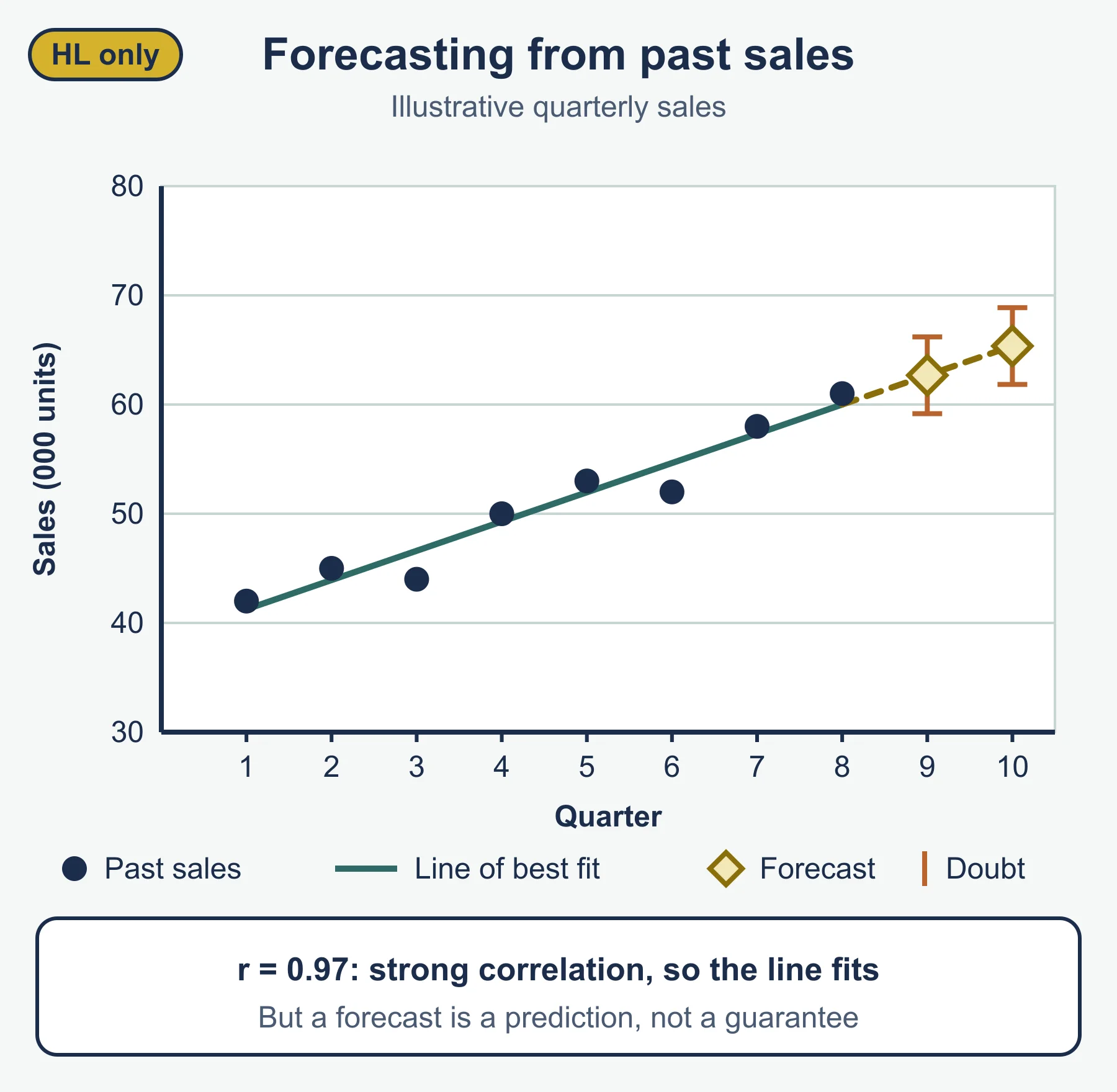
• A line of best fit lets you read off a forecast for a given value of the other variable.
• Correlation is not causation: a third factor may drive both.
• Extrapolation beyond the range of the data is less reliable than reading within it.
• For numerical or graphical data: find the average change or the slope, extend it, state the assumption, interpret the figure in the context of the business.

Responding to forecasts

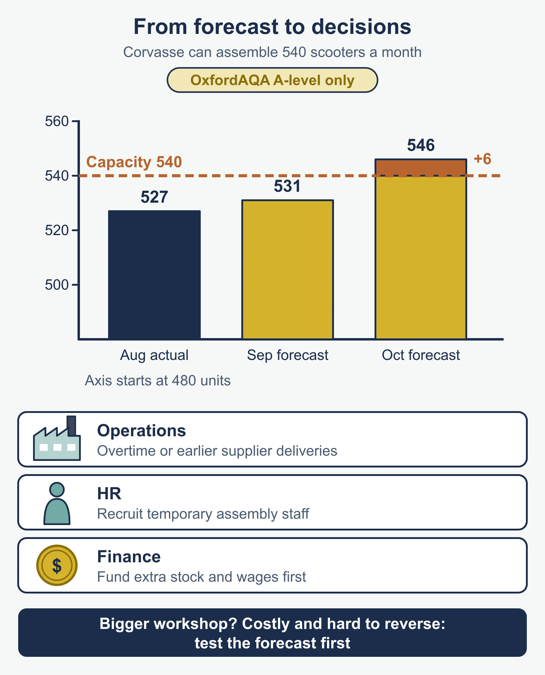
• Match the response to the size of the forecast gap and the cost of acting: adjust production, stock, staffing, prices or finance.
• Examples: arrange an overdraft for a forecast cash shortfall; hire temporary staff for a seasonal peak; delay expansion if the cycle is about to turn.
• To justify, give the reason and compare it with a realistic alternative.
• Importance of accuracy: high when decisions are expensive or hard to reverse, when the lead time is long, or when stakeholders such as lenders rely on the figures.

Quick self-test

1. Define a forecast.
2. Name two structured qualitative methods.
3. Name two unstructured qualitative methods.
4. Annual sales are 50, 56 and 53 (£000) in three consecutive years. Calculate the three-year moving average for the middle year.
5. The actual value is 140 and the trend value is 132. Calculate the cyclical variation.
6. A scatter graph gives a correlation of −0.9. What does that tell you?
7. State one difference between seasonal and cyclical variation.
8. Opening cash is £4,000, cash in is £18,000 and cash out is £20,500. Find the closing balance.
9. A business sells 800 units at £15, with variable cost £9 per unit and fixed costs £4,000. Calculate profit.
10. The trend in 2023 is 130 and rises by 6 a year. Extrapolate the trend for 2026.
11. Give one reason why a moving average cannot be calculated for the latest year.
12. Give one reason why accurate forecasting matters to lenders.

Answers

1. An informed estimate of what will happen to a variable in the future.
2. Delphi technique and expert opinion.
3. Brainstorming and intuition.
4. (50 + 56 + 53) ÷ 3 = 53.0, so £53,000.
5. 140 − 132 = +8, so 8 above trend.
6. Strong negative correlation: as one variable rises, the other tends to fall. It does not prove cause.
7. Seasonal repeats within a year; cyclical spans several years and is irregular in length.
8. 4,000 + 18,000 − 20,500 = £1,500.
9. Revenue 12,000, variable costs 7,200, fixed costs 4,000, so profit is £800.
10. 130 + 3 × 6 = 148.
11. A three-year average needs the following year’s value, which does not exist yet.
12. They rely on cash-flow forecasts to judge whether repayments will be met, so an error raises the risk of default.

Where marks are usually lost

• Describing a method without saying how it is used to forecast.
• Mixing up structured and unstructured methods.
• Writing the moving average against the first year of the three, not the middle one.
• Subtracting the wrong way round for cyclical variation.
• Treating profit and closing cash as the same number.
• Forgetting that opening cash equals the previous month’s closing cash.
• Claiming that correlation proves cause.
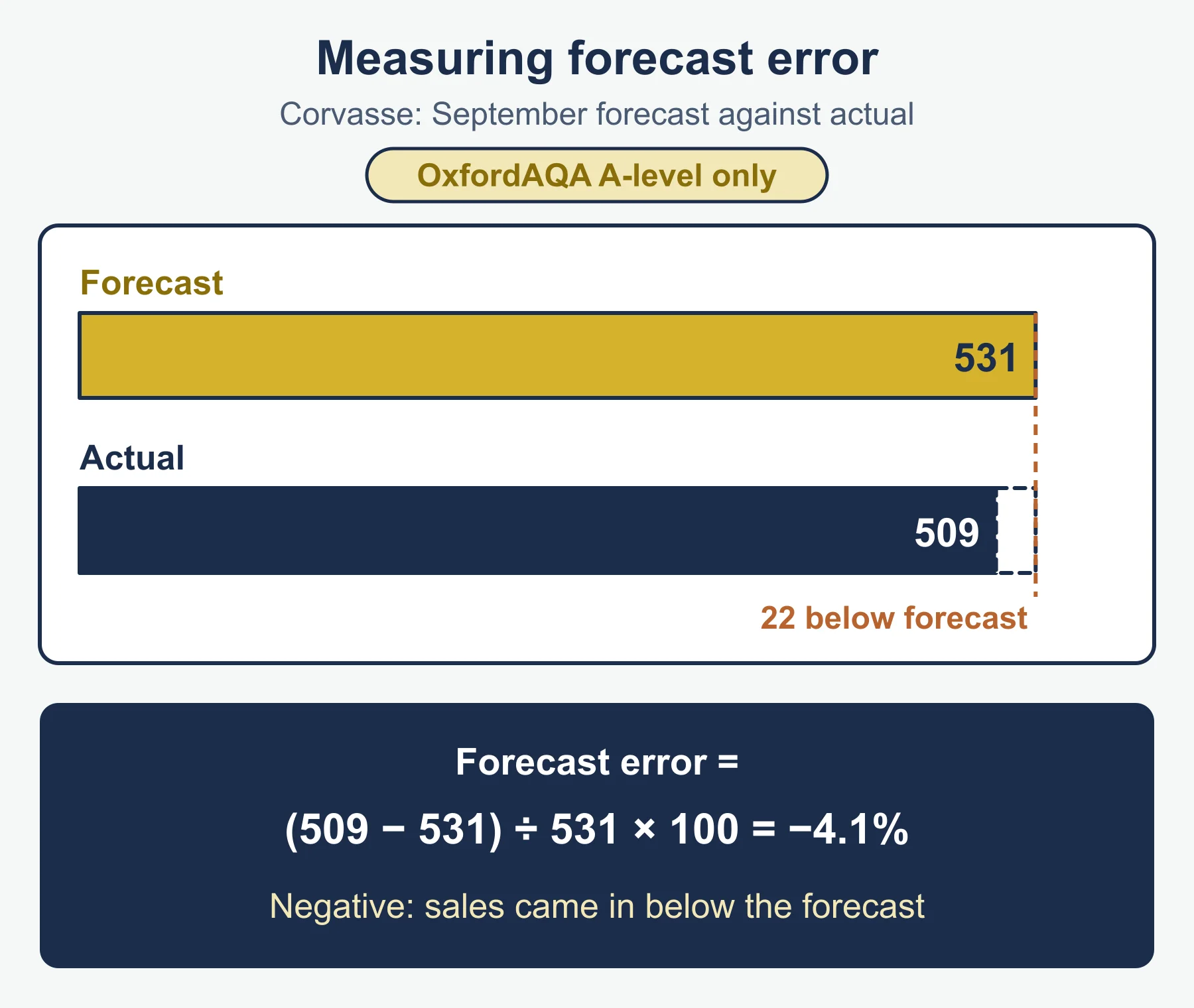
• Giving a forecast as exact, with no comment on assumptions or reliability.
• Listing advantages and disadvantages with no judgement tied to the business in the case.
• Recommending a response with no reason or no comparison with an alternative.

Frequently asked questions

What is the difference between seasonal and cyclical variation? Seasonal variation is a regular, repeating pattern within a year, linked to weather, holidays or the calendar. Cyclical variation is a longer pattern over several years, linked to the economic cycle or an industry cycle of boom, slowdown, recession and recovery.

How do you calculate cyclical variation? Cyclical variation = actual value − trend value, where the trend comes from a moving average. Calculating trend minus actual reverses the sign.

Does correlation prove that one variable causes another? No. Correlation is not causation: a third factor may drive both variables, so treat a forecast based on correlation with care.

What is the difference between qualitative and quantitative forecasting? Qualitative forecasting uses judgement, opinion and experience, and suits a new product with no history. Quantitative forecasting uses numerical data and calculation, such as moving averages and correlation.

Official syllabus

OCR A Level Business (H431), Version 2.1 (January 2026), published by OCR, for first assessment in 2017 with final assessment in summer 2027. Content covered: Forecasting, within the area of study Business objectives and strategy.